Published at 2023-10-03 | Last Update 2023-10-03
借着遇到的一个问题,研究下 loadavg 的算法和实现。
- 1 一次
loadspike 问题排查 - 2
loadavg:算法与内核实现 - 3 讨论
- 4 实用指南
- 5 结束语
- References
查看一台 Linux 机器在过去一段时间的负载
(准确来说是“负载平均”,load average)有很多命令,比如
top、uptime、procinfo、w 等等,
它们底层都是从 procfs 读取的数据:
$ cat /proc/loadavg
0.25 0.23 0.14 1/239 1116826
这是排查 Linux 性能问题时的重要参考指标之一。
proc man page 中有关于它的定义和每一列表示什么的解释:
$ man 5 proc
...
/proc/loadavg
    The first three fields in this file are load average figures giving the number of jobs in the run queue (state R) or waiting for disk I/O (state D) averaged over 1, 5, and 15 minutes.  They are the same as the load average numbers given by uptime(1) and other programs.
    The fourth field consists of two numbers separated by a slash (/).  The first of these is the number of currently runnable kernel scheduling entities (processes, threads).  The value after the slash is the number of kernel scheduling entities that currently exist on the system.
    The fifth field is the PID of the process that was most recently created on the system.
前 3 列分别表示这台机器在过去 1、5、15 分内的负载平均,为方便起见,下文分别用
load1/load5/load15 表示。load1 的精度是这三个里面最高的,
因此本文接下来将主要关注 load1(后面将看到,load5/load15 算法 load1 一样,只是时间尺寸不同)。
需要注意的是,loadavg 是机器的所有 CPU 上所有任务的总负载,因此跟机器的 CPU 数量有直接关系。
CPU 数量不一样的机器,直接比较 loadavg 是没有意义的。为了不同机器之间能够直接对比,
可以将 load1 除以机器的 CPU 数量,得到的指标用 load1_per_core 表示。
有了 load/loadavg 和 load1_per_core 的概念,接下来看一个具体问题。
我们的监控程序会采集每台机器的 load1_per_core 指标。
平时排查问题时经常用这个指标作为性能参考。
1.1 现象
为了定位某个问题,我们对部分 k8s node 加了个 load 告警,比如 load1_per_core > 1.0
就告警出来。加上后前几天平安无事,但某天突然收到了一台机器的告警,它的 load1_per_core 曲线如下:
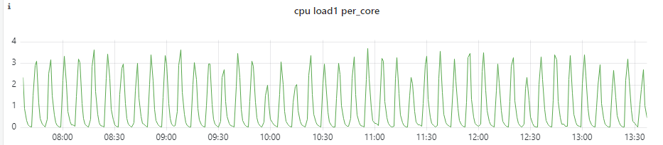
Fig. Load (loadavg1-per-core) spikes of a k8s node
- 对于这些 node,我们预期 load1_per_core 正常不会超过 1,超过 3 就更夸张了;
- 另外,多个业务的 pod 混部在这台机器,根据之前的经验,load 这么高肯定有业务报障, 但这次却没有;
- Load spike 非常有规律,预示着比较容易定位直接原因。
基于以上信息,接下来排查一下。
1.2 排查
1.2.1 宿主机监控:load 和 running 线程数量趋势一致
宿主机基础监控除了 load、cpu、io 等等指标外,我们还采集了系统上的进程/线程、上下文、中断等统计信息。 快速过了一遍这些看板之后发现,load 变化和 node 上总的 running 状态进程数量趋势和时间段都一致:
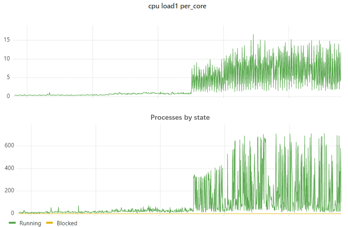
Fig. Node load (load1_per_core) and threads on the node
可以看到 running 进程数量在几十到几百之间剧烈波动。这里的 running 和 blocked 数量采集自:
$ cat /proc/stat
...
procs_running 8
procs_blocked 1
Load 高低和活跃进程数量及 IO 等因素正相关, 因此看到这个监控时,我们首先猜测可能是某些主机进程或 pod 进程在周期性创建和销毁大量进程(线程),或者切换进程(线程)状态。
Linux 调度模块里,实际上是以线程为调度单位(
struct se,schedule entity),并没有进程的概念。
接下来就是找到这个进程或 pod。
1.2.2 定位到进程(Pod)
非常规律的飙升意味着很容易抓现场。登录到 node 先用 top 看了几分钟, 确认系统 loadavg 会周期性从几十飙升到几百,
(node) $ top
#                                                   最近    1      5      15  分钟内的平均总负载
#                                                           |     |      |
top - 16:03:08 up 114 days, 18:03,  1 user,  load average: 17.01, 79.96, 90.27
Tasks: 1137 total,   1 running, 844 sleeping,   0 stopped,   0 zombie
%Cpu(s): 23.3 us,  3.5 sy,  0.0 ni, 72.8 id,  0.0 wa,  0.0 hi,  0.4 si,  0.0 st
...
   PID USER      PR  NI    VIRT    RES    SHR S  %CPU %MEM     TIME+ COMMAND # <-- 进程详情列表
719488 1004      20   0   36.8g   8.5g  35896 S 786.6  3.4  19332:17 java
...
再结合进程详情列表和 %CPU 这一列,很容易确定是哪个进程(PID)引起的,
进而可以根据 PID 找到 Pod。
1.2.3 Pod 监控:大量线程周期性状态切换
找到是哪个 Pod 之后,再跳转到 Pod 监控页面。 我们的监控项中,有一项是 pod 内的任务(线程)数量:
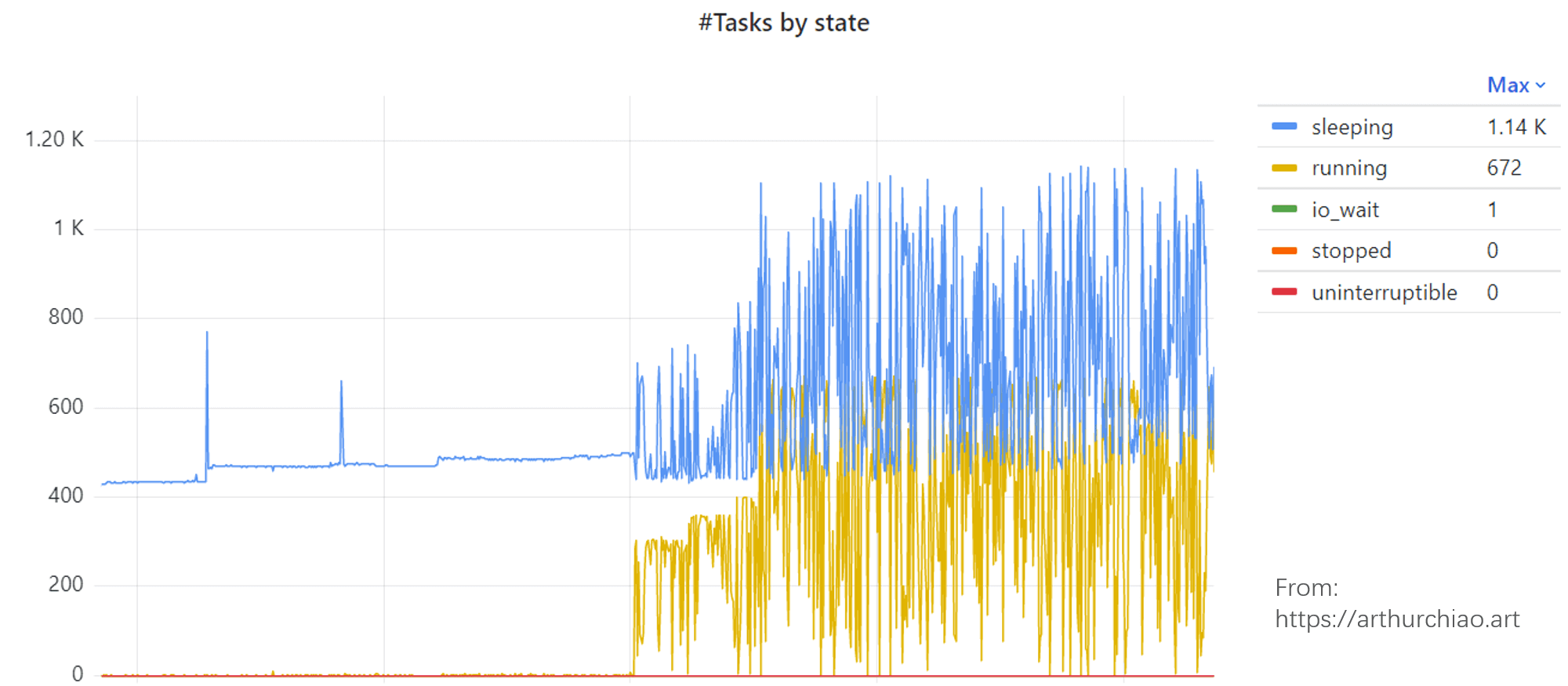
Fig. Task states of the specific Pod
这是在容器内收集的各种状态的线程数量。时间及趋势都和 node 对得上。
再把时间范围拉短了看一下,
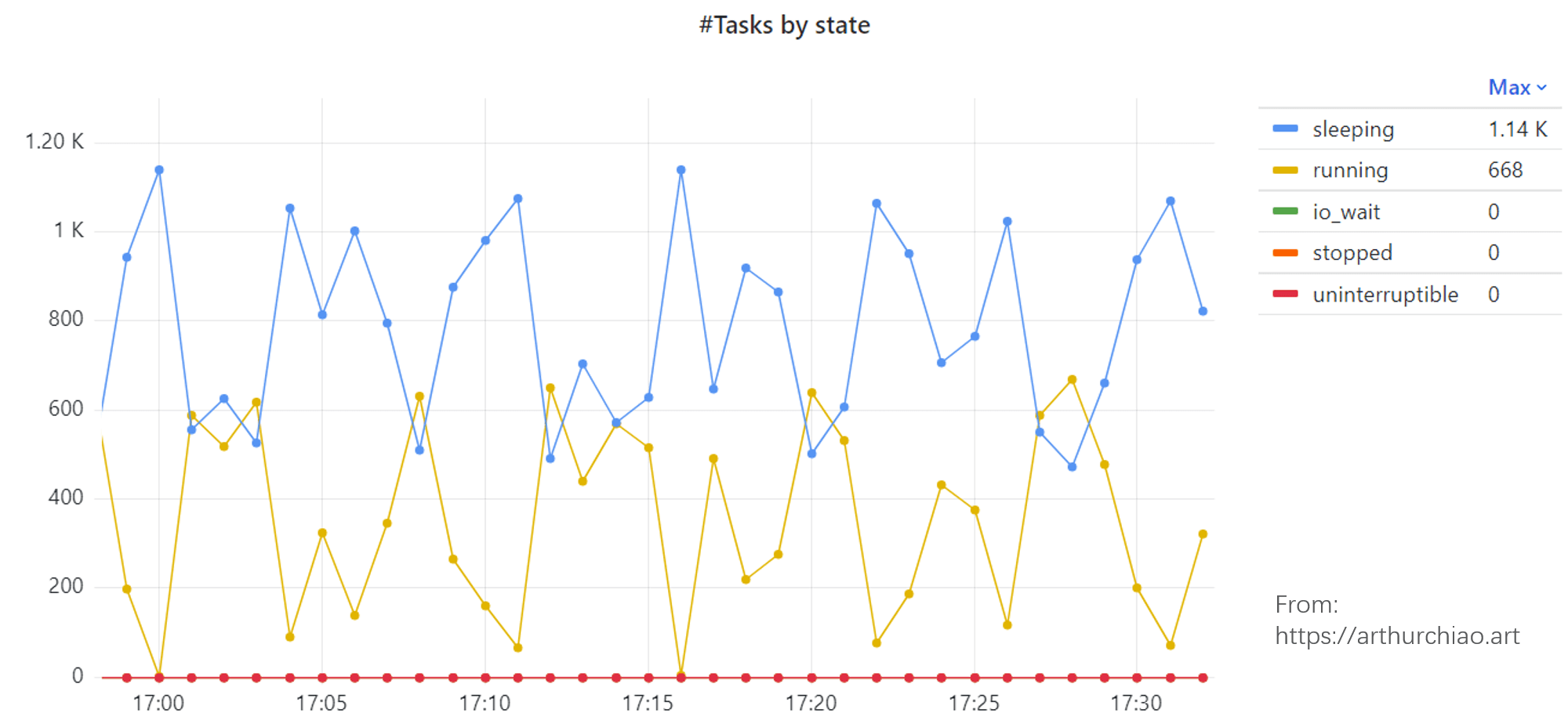
Fig. Task states of the specific Pod
running 线程增多时 sleeping 减少,running 减少时 sleeping 增多,数量对得上。 所以像是 600 来个线程不断在 sleeping/running 状态切换。
1.2.4 交叉验证
计算 loadavg 会用到 Running 和 Uninterrupptable 状态的线程数量, 在 top -H(display individual threads)
里面是 R 和 D 状态,每 5s 统计一次这种线程的数量:
(node) $ for n in `seq 1 30`; do top -b -H -n 1 | egrep "(\sD\s|\sR\s)" | wc -l; sleep 5; done
672
349
106
467
128
378
138
50
453
152
254
701
527
660
695
677
185
32
...
线程数量周期性在 30~700 之间变化,跟监控看到的 load 趋势一致。
其他现象:
mpstat -P ALL 1看了一会,在 load 飙升时只有几个核的 CPU 利用率飙升, 单核最高到 100%;其他 CPU 的利用率都在正常水平;- 每次 load 飙升时,哪些 CPU 的利用率会飙升起来不固定; 这是因为该 Pod 并不是 cpuset 类型,内核会根据 CPU 空闲情况迁移线程;
- IO 没什么变化;
也可以用下面的命令过滤掉那些不会用来计算 load 的线程 (S,T,t,Z,I etc):
$ ps -e -o s,user,cmd | grep ^[RD]
...
1.3 进一步排查方向
根据以上排查,初步总结如下:
- 宿主机 Load 升高是由于 Pod 大量线程进入 running 状态导致的;
- 整体 CPU/IO 等利用率都不高,因此其他业务实际上受影响不大;
进一步排查就要联系业务看看他们的 pod 在干什么了,这个不展开。
1.4 疑问
作为基础设施研发,这个 case 留给我们几个疑问:
- load 到底是怎么计算的?
- load 是否适合作为告警指标?
弄懂了第一个问题,第二个问题也就有答案了。 因此接下来我们研究下第一个问题。
接下来的代码基于内核 5.10。
2.1 原理与算法
loadavg 算法本质上很简单,但 Linux 内核为了减少计算开销、适配不同处理器平台等等,做了很多工程优化, 所以现在很难快速看懂了。算法实现主要在 kernel/sched/loadavg.c [4], 上来就是官方吐槽:
This file contains the magic bits required to compute the global loadavg figure. Its a silly number but people think its important. We go through great pains to make it work on big machines and tickless kernels.
吐槽结束之后是算法描述:
The global load average is an exponentially decaying average of nr_running + nr_uninterruptible.

Once every LOAD_FREQ:

  nr_active = 0;
  for_each_possible_cpu(cpu)
      nr_active += cpu_of(cpu)->nr_running + cpu_of(cpu)->nr_uninterruptible;

  avenrun[n] = avenrun[0] * exp_n + nr_active * (1 - exp_n)
其中的 avenrun[] 就是 loadavg。这段话说,
- loadavg 是
nr_running + nr_uninterruptible状态线程数量的一个指数衰减平均; - 算法每隔
5s(LOAD_FREQ)根据公式计算一次过去 n 分钟内的 loadavg,其中 n 有三个取值:1/5/15; - 对于 1 分钟粒度的 loadavg,公式简化为
avenrun[n] = avenrun[0] * exp_1 + nr_active * (1 - exp_1)。
根据 [3],最近 1 分钟的 load 计算公式可以进一步精确为:
load(t) = load(t-1)e-5/60 + nr_active * (1-e-5/60) 公式 (1)
其中的参数:
t:时刻;nr_active:所有 CPU 上 nr_running + nr_uninterruptible 的 task 数量;
根据 nr_active 的取值,又分为两种情况,下面分别来看。
2.1.1 有活跃线程:load 指数增长
nr_active > 0 表示此时(至少一个 CPU 上)有活跃线程。此时(尤其是活跃线程比较多时),
公式 1 的后面一部分占主,前面的衰减部分可以忽略,公式简化为:
load(tT) = nr_active * load(t0)(1-e-5t/60) 公式 (2)
t0 是初始时刻,tT 是 T 时刻。
可以看出,这是一个与 nr_active 呈近似线性的单调递增曲线。
2.1.2 无活跃线程:load 指数衰减
nr_active = 0 表示所有 CPU 上都没有活跃线性,即整个系统处于空闲状态。
此时,公式简化为:
load(tT) = load(t0)e-5t/60 公式 (3)
是一个标准的指数衰减。也就是说如果从此刻开始, 后面都没有任务运行了,那系统 load 将指数衰减下去。
2.1.3 Load 测试与小结
我们来快速验证下。
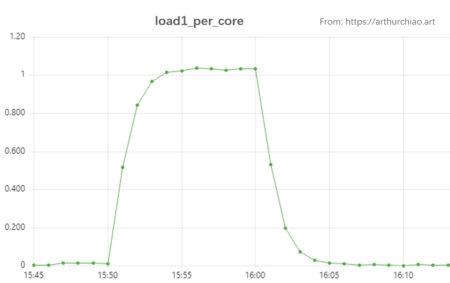
在一台 48 核机器上,创建 44 个线程(留下 4 个核跑系统任务,比如监控采集程序)压测 10 分钟:
# spawn 44 workers spinning on malloc()/free(), run for 10 minutes
$ stress -m 44 --timeout 600s
下面是 load1_per_core 的监控:

Fig. Load test on a 48-Core physical server. stress -m 44 --timeout 600s
Load 曲线明显分为两个阶段:
15:50~16:00,一直有 44 个活跃线性,因此 load 一个单调递增曲线,前半部分近似线性(后面为什么越来越平了?);16:00~16:10,没有活跃线性(除了一些开销很小的系统线程),因此 load 是一个比较标准的指数衰减曲线;
注意:
- 图中纵轴的单位是 load1_per_core,乘以这台机器的核数 48 才是 loadavg,也就是公式 1-3 中的 load。 不过由于二者就差一个固定倍数,因此曲线走势是一模一样的。
- 后面会看到,内核每
5s计算一次 load,而这里的监控是每60s采集一个点,所以曲线略显粗糙;如果有精度更高的采集(例如,也是 5s 采集一次),会看到一条更漂亮的曲线。 - 另外注意注意到 load1_per_core 最大值已经超过 1 了,因此它并不是一个
<= 1.0 (100%)的指标, 活跃线程数量越多,load 就越大。如果压测时创建更多的活跃线性,就会看到 load 达到一个更大的平稳值。 它跟 CPU 利用率(最大 100%)并不是一个概念。
有了这样初步的感性认识之后,接下来看看内核实现。
2.2 内核基础
要大致看懂代码,需要一些内核基础。
2.2.1 运行/调度队列 struct rq
内核在每个 CPU 上都有一个调度队列,叫 runqueue(运行队列),
对应的结构体是 struct rq。
这是一个通用调度队列,里面包含了大量与调度相关的字段,比如
完全公平调度器
struct cfs_rq cfs。
本文主要关注的是与计算 load 有关的几个字段,
// kernel/sched/sched.h

// This is the main, per-CPU runqueue data structure.
struct rq {
    unsigned int         nr_running;        // running task 数量
    struct   cfs_rq      cfs;               // 完全公平调度器 CFS

    unsigned long        nr_uninterruptible;// 不可中断状态的 task 数量

    // 与 load 计算相关的字段
    unsigned long        calc_load_update;  // 上次计算 load 的时刻
    long                 calc_load_active;  // 上次计算 load 时的 nr_active (running+uninterruptible)
    ...
};
如上,有两个 calc_load_ 前缀的变量,表明这是计算 load 用的,
后缀表示变量的用途,
calc_load_update:上次计算 load 的时刻;calc_load_tasks:上次计算 load 时的 running+uninterruptible 状态的 task 数量(内核代码中 task 表示的是一个进程或一个线程);
代码中看到这俩变量时,可能觉得更像是函数名而不是变量。如果更倾向于可读性,这俩变量可以改为:
- prev_load_calc_time
- prev_load_calc_active_tasks 或 prev_load_calc_nr_active
2.2.2 Load 计算相关的全局变量
计算 load 用的几个全局变量:
// kernel/sched/loadavg.c

atomic_long_t calc_load_tasks;  // CPU 上 threads 数量
unsigned long calc_load_update; // 时间戳
unsigned long avenrun[3];
- 前两个跟 runqueue 里面的字段对应,但计算的是所有 CPU 上所有 runqueue 对应字段的总和, 因为 load 表示是系统负载,不是单个 CPU 的负载。
- 第三个变量
avenrun[3]前面也看到了,表示的是过去 1、5、15 分钟内的 loadavg。
2.2.3 内核时间基础:HZ/tick/jiffies/uptime
Linux 内核的周期性事件基于 timer interrupt
触发,计时基于 HZ,这是一个编译常量,通常与 CPU 架构相关。
例如,对于最常见的 X86 架构,
- 默认 HZ 是
1000,也就是 1s 内触发 1000 次 timer interrupt,interrupt 间隔是1s/HZ = 1ms; 这和处理器的晶振频率(例如2.1G HZ)并不是一个概念,别搞混了; -
在计时上,一次 timer interrupt 也称为一次
tick,- tick 的间隔称为
tick period,因此有 tick period =1s/HZ; - 在内核中有两个相关变量
// kernel/time/tick-common.c // Tick next event: keeps track of the tick time ktime_t tick_next_period; ktime_t tick_period; // Setup the tick device static void tick_setup_device(struct tick_device *td, struct clock_event_device *newdev, int cpu, const struct cpumask *cpumask) { tick_next_period = ktime_get(); tick_period = NSEC_PER_SEC / HZ; // 内部用 ns 表示 } - tick 的间隔称为
-
系统启动以来的 tick 次数记录在全局变量
jiffies里面,// linux/jiffies.h extern unsigned long volatile jiffies;系统启动时初始化为 0,每次 timer interrupt 加 1。由于 timer interrupt 是 1ms, 因此 jiffies 就是以 1ms 为单位的系统启动以来的时间。 jiffies_64 是 64bit 版本的 jiffies。
-
jiffies 和 uptime 的关系:
uptime_in_seconds = jiffies / HZ以及
jiffies = uptime_in_seconds * HZ
有了以上基础,接下来可以看算法实现了。
2.3 算法实现
2.3.1 调用栈
每次 timer interrupt 之后,会执行到 tick_handle_periodic(),接下来的调用栈:
tick_handle_periodic // kernel/time/tick-common.c
  |-cpu = smp_processor_id();
  |-tick_periodic(cpu)
      |-if (tick_do_timer_cpu == cpu) { // 只有一个 CPU 负责计算 load,不然就乱套了
      |   tick_next_period = ktime_add(tick_next_period, tick_period); // 更新全局变量
      |   do_timer(ticks=1)
      |   | |-jiffies_64 += ticks; // 都是 ns 表示的
      |   | |-calc_global_load();
      |   |     | // update the avenrun load estimates 10 ticks after the CPUs have updated calc_load_tasks.
      |   |     |-if jiffies < calc_load_update + 10
      |   |     |   return;
      |   |     |
      |   |     |-active = atomic_long_read(&calc_load_tasks);
      |   |     |-active = active > 0 ? active * FIXED_1 : 0;
      |   |     |-avenrun[0] = calc_load(load=avenrun[0], exp=EXP_1, active);
      |   |     |                |-newload = avenrun[0] * EXP_1 + active * (FIXED_1 - EXP_1)
      |   |     |                |-if (active >= avenrun[0])
      |   |     |                |     newload += FIXED_1-1;
      |   |     |                |
      |   |     |                |-return newload / FIXED_1;
      |   |     |
      |   |     |-avenrun[1] = calc_load(avenrun[1], EXP_5, active);
      |   |     |-avenrun[2] = calc_load(avenrun[2], EXP_15, active);
      |   |     |-WRITE_ONCE(calc_load_update, sample_window + LOAD_FREQ); // 下一次计算 loadavg 的时间:5s 后
      |   |     |
      |   |     |-calc_global_nohz(); // In case we went to NO_HZ for multiple LOAD_FREQ intervals catch up in bulk.
      |   |         |-calc_load_n
      |   |             |-calc_load
      |   |
      |   update_wall_time()
      |-}
      |-update_process_times(user_mode(get_irq_regs()));
      |-profile_tick(CPU_PROFILING);
timer 中断之后,执行 tick_handle_periodic(),它首先
获取程序当前所在的 CPU ID,然后执行 tick_periodic(cpu)。
接下来的大致步骤:
- 判断是不是当前 CPU 负责计算 load,是的话才继续;否则只更新一些进程 timer 信息就返回了;
- 如果是当前 CPU 负责计算,则更新下次 tick 时间戳 tick_next_period,也就是在当前时间基础上加上 tick_period (1/HZ 秒,x86 默认是 1ms);
- 调用
do_timer(ticks=1)尝试计算一次 load;这里说尝试是因为不一定真的会计算,可能会提前返回; -
更新 jiffies_64;然后计算 load,
如果 jiffies 比上次计算 load 的时间戳 + 10 要小,就不计算; 否则,调用
calc_load()开始计算 loadavg。
计算 load 的算法就是我们上一节介绍过的了:
The global load average is an exponentially decaying average of nr_running + nr_uninterruptible.

Once every LOAD_FREQ(5 秒):

  nr_active = 0;
  for cpu in cpus:
      nr_active += cpu->nr_running + cpu->nr_uninterruptible;

  avenrun[n] = avenrun[0] * exp_n + nr_active * (1 - exp_n)
2.3.2 一些实现细节
runqueue load 字段初始化
static void sched_rq_cpu_starting(unsigned int cpu) {
    struct rq *rq = cpu_rq(cpu);

    rq->calc_load_update = calc_load_update;
    update_max_interval();
}

void __init sched_init(void) {
    for_each_possible_cpu(i) {
        struct rq *rq;

        rq = cpu_rq(i);
        raw_spin_lock_init(&rq->lock);
        rq->nr_running = 0;
        rq->calc_load_active = 0;
        rq->calc_load_update = jiffies + LOAD_FREQ;
    }
}
判断是否由当前 CPU 执行 load 计算
// kernel/time/tick-common.c

/*
 * tick_do_timer_cpu is a timer core internal variable which holds the CPU NR
 * which is responsible for calling do_timer(), i.e. the timekeeping stuff. This
 * variable has two functions:
 *
 * 1) Prevent a thundering herd issue of a gazillion of CPUs trying to grab the
 *    timekeeping lock all at once. Only the CPU which is assigned to do the
 *    update is handling it.
 *
 * 2) Hand off the duty in the NOHZ idle case by setting the value to
 *    TICK_DO_TIMER_NONE, i.e. a non existing CPU. So the next cpu which looks
 *    at it will take over and keep the time keeping alive.  The handover
 *    procedure also covers cpu hotplug.
 */
int tick_do_timer_cpu __read_mostly = TICK_DO_TIMER_BOOT;
do_timer()
// kernel/time/tick-common.c

// kernel/time/timekeeping.c
void do_timer(unsigned long ticks) {
    jiffies_64 += ticks;
    calc_global_load();
}
calc_global_load() -> calc_load()
// kernel/time/tick-common.c

/*
 * calc_load - update the avenrun load estimates 10 ticks after the
 * CPUs have updated calc_load_tasks.
 *
 * Called from the global timer code.
 */
void calc_global_load(void) {
    unsigned long sample_window;
    long active, delta;

    sample_window = READ_ONCE(calc_load_update);
    if (time_before(jiffies, sample_window + 10))
        return;

    /*
     * Fold the 'old' NO_HZ-delta to include all NO_HZ CPUs.
     */
    delta = calc_load_nohz_read();
    if (delta)
        atomic_long_add(delta, &calc_load_tasks);

    active = atomic_long_read(&calc_load_tasks);
    active = active > 0 ? active * FIXED_1 : 0;

    avenrun[0] = calc_load(avenrun[0], EXP_1, active);
    avenrun[1] = calc_load(avenrun[1], EXP_5, active);
    avenrun[2] = calc_load(avenrun[2], EXP_15, active);

    WRITE_ONCE(calc_load_update, sample_window + LOAD_FREQ);

    /*
     * In case we went to NO_HZ for multiple LOAD_FREQ intervals
     * catch up in bulk.
     */
    calc_global_nohz();
}

/*
 * a1 = a0 * e + a * (1 - e)
 */
static inline unsigned long
calc_load(unsigned long load, unsigned long exp, unsigned long active) {
    unsigned long newload = load * exp + active * (FIXED_1 - exp);
    if (active >= load)
        newload += FIXED_1-1;

    return newload / FIXED_1;
}
2.4 考古
[2] 中对 Linux loadavg 算法演变做了一些考古。 主要是关于 Linux 为什么计算 loadavg 时需要考虑到 uninterruptible sleep 线程数量, 以及 Linux 的 loadavg 和其他操作系统的 loadavg 有什么区别。
2.4.1 计入不可中断 sleep
Uninterruptible Sleep (D) 状态通常是同步 disk IO 导致的 sleeping;
- 这种状态的 task 不受中断信号影响,例如阻塞在 disk IO 和某些 lock 上的 task;
- 将这种状态的线性引入 loadavg 计算的 patch;
- 使得 Linux 系统 loadavg 表示的不再是 “CPU load averages”,而是 “system load averages”。
2.4.2 Linux vs. 其他 OS:loadavg 区别
Linux load 与其他操作系统 load 的区别: 几点重要信息:
| 操作系统 | load average 概念和内涵 | 优点 |
|---|---|---|
| Linux | 准确说是 system load average,衡量的是系统整体资源,而非 CPU 这一种资源。包括了正在运行和等待(CPU, disk, uninterruptible locks 等资源)运行的所有线程数量,换句话说,统计所有非完全空闲的线程(threads that aren’t completely idle)数量 |
考虑到了 CPU 之外的其他资源 |
| 其他操作系统 | 指的就是 CPU load average,衡量所有 CPU 上 running+runnable 线程的数量 |
理解简单,也更容易推测 CPU 资源的使用情况 |
3.1 Load 很高,所有进程都会受影响吗?
不一定。
Load 是根据所有 CPU 的 runqueue
状态综合算出的一个数字,load 很高并不能代表每个 CPU 都过载了。
例如,少数几个 CPU 上有大量或持续活跃线程,就足以把系统 load 打到很高, 但这种情况下,其他 CPU 上的任务并不受影响。下面来模拟一下。
3.1.1 模拟:单个 CPU 把系统 load 打高上百倍
下面是一台 4C 空闲机器上,
$ cat /proc/cpuinfo | grep processor
processor       : 0
processor       : 1
processor       : 2
processor       : 3

$ uptime
 16:52:13 up  3:15,  7 users,  load average: 0.22, 0.18, 0.18
系统 loadavg1 只有 0.22。接下来创建 30 个 stress 任务并固定到 CPU 3 上执行,
# spawn 30 workers spinning on sqrt()
$ taskset -c 3 stress -c 30 --timeout 120s
然后通过 top 命令 5s 查看一次 loadavg1:
$ for n in `seq 1 120`; do top -b -n1 | head -n1 | awk '{print $(NF-2)}' | sed 's/,//'; sleep 5; done
0.24
0.22
0.26
2.64
4.84
6.85
8.70
10.41
11.98
13.42
14.75
15.97
17.09
18.13
19.08
19.95
20.76
21.50
22.18
22.81
23.38
23.91
24.40
24.85
25.26
25.64
25.99
23.91
可以看到,loadavg 最高到了 25 以上,比我们压测之前高了 100 多倍。 看一下压测期间的 CPU 利用率:
$ mpstat -p ALL 1
Average:  CPU    %usr  %nice   %sys %iowait   %irq  %soft  %steal  %guest  %gnice   %idle
Average:  all   25.02   0.00   0.17    0.00   0.00   0.00    0.00    0.00    0.00   74.81
Average:    0    0.00   0.00   0.33    0.00   0.00   0.00    0.00    0.00    0.00   99.67 # -+
Average:    1    0.00   0.00   0.33    0.00   0.00   0.00    0.00    0.00    0.00   99.67 #  | CPU 0-2 are idle
Average:    2    0.00   0.00   0.00    0.00   0.00   0.00    0.00    0.00    0.00  100.00 # -+
Average:    3  100.00   0.00   0.00    0.00   0.00   0.00    0.00    0.00    0.00    0.00
           #      |
           # CPU 3 is 100% busy
可以看到只有 CPU 3 维持在 100%,其他几个 CPU 都是绝对空闲的。
3.1.2 cpuset vs. cpu quota
假如我们的压测程序是跑在一个 pod 里,这种情况对应的就是 cpuset
模式 —— 独占几个固定的 CPU。这种情况下除了占用这些 CPU 的 Pod 自身,其他 Pod 是不受影响的
(单就 CPU 这一种资源来说。实际上 pod 还共享其他资源,例如宿主机的总网络带宽、IO 等)。
非 cpuset 的 pod 没有独占 CPU,系统通过 cgroup/cfs 来分配给它们 CPU 份额, 线程也会在 CPU 之间迁移,因此影响其他 pod 的可能性大一些。一些相关内容:
3.2 僵尸进程
loadavg 也会计入僵尸进程(Z 状态),因此如果有大量僵尸进程,也会看到系统的 load 很高。
3.3 Load != CPU 利用率
loadavg 衡量系统整体在过去一段时间内的负载状态,
- 每 5s 对所有 CPU 上所有 runqueue 采样一次,本质上表示的是 runqueue length,并不是 CPU 利用率;
- 是一种 指数衰减移动平均(exponentially-damped moving average);
CPU 利用率统计的是 CPU 繁忙的时间占比,比如对于单个 CPU,
- 在 1s 的周期内有 0.5s 在执行任务,剩下的时间是空闲的,那 CPU 利用率就是 50%;
- 利用率上限是 100%;
3.4 Load 是否是一个很好的告警指标?
根据以上讨论,load 高并不一定表示每个 CPU 都繁忙。极端情况下,单核或单个应用的线程太多就能导致 load 飙升成百上千倍, 但这时可能除了少数几个核,其他核上的应用都不受影响,所以用 load 来告警并不合适; 更准确的是每个 CPU 独立计算 load,即 per-core-loadavg,但目前并没有这个指标。
但另一方面,load 趋势变化在实际排障中还是很有参加价值的, 比如之前 loadavg 是 0.5,现在突然变成 0.8,那说明系统任务数量或状态还是有较大变化的, 为进一步排查指明了一个方向。
既然 load 只能用来看趋势和相对大小,判断是否可能有问题,而无法及衡量问题的严重程度及进一步定位问题根源, 那怎么进一步排查和定位问题呢?下面是一些参考。
4.1 USE (Used-frequency, Saturation, Errors) 方法论
《Systems Performance: Enterprise and the Cloud》(中文版名为《性能之巅》)一书提出了 衡量一种资源使用状况的 3 个维度的指标 [5]:
- 利用率(Utilization): 例如,CPU 利用率
90%(有90%的时间内,这个 CPU 有被使用到); - 饱和度(Saturation): 用 wait-queue length 衡量,例如,CPU 的平均
runqueue length是 4; - 错误数(Errors): 例如网卡有 50 个丢包
但 [7] 中已经分析过,USE 术语给 “Utilization” 这个词带来了相当大的歧义,因为大家说到 “utilization”(“利用率”) 时,普遍指的是一种资源总共被使用了多少 —— 比如我有 4 个 CPU,其中 3 个 100% 在运行,那 “utilization” 就是 75% —— 这对应的其实是 USE 里面的 “saturation”(“饱和度”)概念。作者重新将 “Utilization” 定义为“使用频率” —— 在采样周期内,有多长时间这种资源有被使用到(不管使用了多少) —— 给一个已经普遍接受的术语重新定义概念,造成很大的理解和交流障碍。 为此,本文把 USE 中的 “U” 解释成 “Used-frequency”。方法论没有任何变化,只是改个术语来减少混淆。
举例,对于一片 100 核的 GPU,
- Used-frequency:在采样周期内,这种资源被使用到的时间比例;例如采样周期是 1s, 其中 0.8s 的时间内有至少有一个核在执行计算,那 U 就是 80%; 实际用了几个核,从这个指标推测不出来;
- Saturation:
100% * used_cores / total_cores;这个指标可以推测平均用了几个核; - Errors:(一般是 Saturation 超过一定阈值之后,)这个 GPU 的报错数量。
4.2 指标
进一步排查,可以参考下列 U 和 S 指标。
4.2.1 Used-frequency 指标
在定义 workload 行为特征方面比较有用,
per-CPUused-frequency:mpstat -P ALL 1;per-processCPU used-frequency: eg, top,pidstat 1。
4.2.2 Saturation 指标
在瓶颈分析方面比较有用:
-
Per-CPU 调度延迟(CPU run queue
latency)-
/proc/schedstat$ cat /proc/schedstat version 15 timestamp 4300445966 cpu0 0 0 0 0 0 0 1251984973307 142560271674 30375313 cpu1 0 0 0 0 0 0 1423130608498 155128353435 40480095 cpu2 0 0 0 0 0 0 1612417112675 603370909483 43658159 cpu3 0 0 0 0 0 0 1763144199179 4220860238053 31154491 perf sched- bcc
runqlat脚本
-
-
全局调度队列长度(CPU run queue
length): 这个指标能看出有没有问题,但是很难估计问题的严重程度。-
vmstat 1,看r列的数据;$ vmstat 1 procs -----------memory---------- ---swap-- -----io---- -system-- ------cpu----- r b swpd free buff cache si so bi bo in cs us sy id wa st 2 0 220532 69004 56416 1305500 1 10 387 370 900 1411 9 2 89 0 0 0 0 220532 69004 56416 1305700 0 0 0 0 774 1289 0 1 99 0 0 ... -
bcc
runqlen脚本
-
-
Per-thread run queue (scheduler) latency: 这是最好的 CPU 饱和度指标,它表示 task/thread 已经 runnable 了,但是还没有等到它的时间片; 可以计算出一个线程花在 scheduler latency 上的时间百分比。这个比例很容易量化,看出问题的严重程度。 具体指标:/proc/PID/schedstatsdelaystatsperf sched
本文从遇到的具体问题出发,研究了一些 Linux load 相关的内容。 一些内容和理解都还比较粗糙,后面有机会再完善。
- High System Load with Low CPU Utilization on Linux?, tanelpoder.com, 2020
- Linux Load Averages: Solving the Mystery, brendangregg.com, 2017
- UNIX Load Average Part 1: How It Works, fortra.com
- kernel/sched/loadavg.c, 2021
- (笔记)《Systems Performance: Enterprise and the Cloud》(Prentice Hall, 2013), 2020
- Linux Trouble Shooting Cheat Sheet, 2020
- Understanding NVIDIA GPU Performance: Utilization vs. Saturation (2023)
如有侵权请联系:admin#unsafe.sh