[译][论文] BERT：预训练深度双向 Transformers 做语言理解（Google，2019）

[译][论文] BERT：预训练深度双向 Transformers 做语言理解（Google，2019）
2024-3-10 08:0:0 Author: arthurchiao.github.io(查看原文) 阅读量:81 收藏

Published at 2024-03-10 | Last Update 2024-03-10

译者序

本文翻译自 2019 年 Google 的论文： BETT: Pre-training of Deep Bidirectional Transformers for Language Understanding。

@article{devlin2018bert,
  title={BERT: Pre-training of Deep Bidirectional Transformers for Language Understanding},
  author={Devlin, Jacob and Chang, Ming-Wei and Lee, Kenton and Toutanova, Kristina},
  journal={arXiv preprint arXiv:1810.04805},
  year={2018}
}

与 GPT 一样，BERT 也基于 transformer 架构，从诞生时间来说，它位于 GPT-1 和 GPT-2 之间，是有代表性的现代 transformer 之一，现在仍然在很多场景中使用，

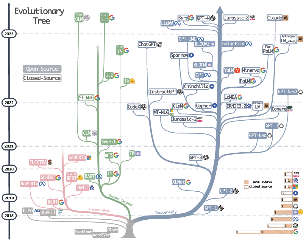
大模型进化树，可以看到 BERT 所处的年代和位置。图来自大语言模型（LLM）综述与实用指南（Amazon，2023）。

根据 Transformer 是如何工作的：600 行 Python 代码实现两个（文本分类+文本生成）Transformer（2019）， BERT 是首批 在各种自然语言任务上达到人类水平的 transformer 模型之一。预训练和 fine-tuning 代码：github.com/google-research/bert。

BERT 模型只有 0.1b ~ 0.3b 大小，因此在 CPU 上也能较流畅地跑起来。

译者水平有限，不免存在遗漏或错误之处。如有疑问，敬请查阅原文。

以下是译文。

译者序
摘要
1 引言
2 相关工作
3 BERT
4 实验
5 对照研究
6 总结
附录
参考文献

本文提出 BERT（Bidirectional Encoder Representations from Transformers， 基于 Transformers 的双向 Encoder 表示） —— 一种新的语言表示模型（language representation model）。

与最近的语言表示模型（Peters 等，2018a; Radford 等，2018）不同， BERT 利用了所有层中的左右上下文（both left and right context in all layers），在无标签文本（unlabeled text）上 预训练深度双向表示（pretrain deep bidirectional representations）。
只需添加一个额外的输出层，而无需任何 task-specific 架构改动，就可以对预训练的 BERT 模型进行微调，创建出用于各种下游任务（例如问答和语言推理）的高效模型。

BERT 在概念上很简单，实际效果却很强大，在 11 个自然语言处理任务中刷新了目前业界最好的成绩，包括，

GLUE score to 80.5% (7.7% point absolute improvement)
MultiNLI accuracy to 86.7% (4.6% absolute improvement)
SQuAD v1.1 question answering Test F1 to 93.2 (1.5 point absolute improvement)
SQuAD v2.0 Test F1 to 83.1 (5.1 point absolute improvement)

业界已证明，语言模型预训练（Language model pre-training）能显著提高许多自然语言处理（NLP）任务的效果（Dai 和 Le，2015; Peters 等，2018a; Radford 等，2018; Howard 和 Ruder，2018）。这些任务包括：

sentence-level tasks：例如自然语言推理（Bowman 等，2015; Williams 等，2018）；
paraphrasing（Dolan 和 Brockett，2005）：整体分析句子来预测它们之间的关系；
token-level tasks：例如 named entity recognition 和问答，其模型需要完成 token 级别的细粒度输出（Tjong Kim Sang 和 De Meulder，2003; Rajpurkar 等，2016）。

1.1 Pre-trained model 适配具体下游任务的两种方式

将预训练之后的语言表示（pre-trained language representations）应用到下游任务，目前有两种策略：

基于特征的方式（feature-based approach）：例如 ELMo（Peters 等，2018a），使用任务相关的架构，将预训练表示作为附加特征。
微调（fine-tuning）：例如 Generative Pre-trained Transformer (OpenAI GPT)（Radford 等，2018），引入最少的 task-specific 参数，通过微调所有预训练参数来训练下游任务。

这两种方法都是使用单向语言模型来学习通用语言表示。

1.2 以 OpenAI GPT 为代表的单向架构存在的问题

我们认为，以上两种方式（尤其是微调）限制了 pre-trained language representation 的能力。主要是因为其语言模型是单向的，这限制了预训练期间的架构选择范围。

例如，OpenAI GPT 使用从左到右的架构（Left-to-Right Model, LRM），因此 Transformer self-attention 层中的 token 只能关注它前面的 tokens（只能用到前面的上下文）：

对于句子级别的任务，这将导致次优结果；
对 token 级别的任务（例如问答）使用 fine-tuning 方式效果可能非常差，因为这种场景非常依赖双向上下文（context from both directions）。

1.3 BERT 创新之处

本文提出 BERT 来改进基于微调的方式。

受 Cloze（完形填空）任务（Taylor，1953）启发，BERT 通过一个“掩码语言模型”（masked language model, MLM）做预训练，避免前面提到的单向性带来的问题，

MLM 随机掩盖输入中的一些 token ，仅基于上下文来预测被掩盖的单词（单词用 ID 表示）。
与从左到右语言模型的预训练不同，MLM 能够同时利用左侧和右侧的上下文，从而预训练出一个深度双向 Transformer。

除了掩码语言模型外，我们还使用“下一句预测”（next sentence prediction, NSP）任务来联合预训练 text-pair representation。

1.4 本文贡献

证明了双向预训练对于语言表示的重要性。与 Radford 等（2018）使用单向模型预训练不同，BERT 使用掩码模型来实现预训练的深度双向表示。这也与 Peters 等（2018a）不同，后者使用独立训练的从左到右和从右到左的浅连接。
展示了 pre-trained representations 可以减少对许多 task-specific 架构的重度工程优化。 BERT 是第一个在大量 sentence-level 和 token-level 任务上达到了 state-of-the-art 性能的 基于微调的表示模型，超过了许多 task-specific 架构。
BERT 刷新了 11 个自然语言处理任务的最好性能。

代码和预训练模型见 github.com/google-research/bert。

（这节不是重点，不翻译了）。

There is a long history of pre-training general language representations, and we briefly review the most widely-used approaches in this section.

2.1 无监督基于特征（Unsupervised Feature-based）的方法

Learning widely applicable representations of words has been an active area of research for decades, including non-neural (Brown et al., 1992; Ando and Zhang, 2005; Blitzer et al., 2006) and neural (Mikolov et al., 2013; Pennington et al., 2014) methods. Pre-trained word embeddings are an integral part of modern NLP systems, offering significant improvements over embeddings learned from scratch (Turian et al., 2010). To pretrain word embedding vectors, left-to-right language modeling objectives have been used (Mnih and Hinton, 2009), as well as objectives to discriminate correct from incorrect words in left and right context (Mikolov et al., 2013).

These approaches have been generalized to coarser granularities, such as

sentence embeddings (Kiros et al., 2015; Logeswaran and Lee, 2018)
paragraph embeddings (Le and Mikolov, 2014).

To train sentence representations, prior work has used objectives to rank candidate next sentences (Jernite et al., 2017; Logeswaran and Lee, 2018), left-to-right generation of next sentence words given a representation of the previous sentence (Kiros et al., 2015), or denoising autoencoder derived objectives (Hill et al., 2016).

ELMo and its predecessor (Peters et al., 2017, 2018a) generalize traditional word embedding research along a different dimension. They extract context-sensitive features from a left-to-right and a right-to-left language model. The contextual representation of each token is the concatenation of the left-to-right and right-to-left representations. When integrating contextual word embeddings with existing task-specific architectures, ELMo advances the state of the art for several major NLP benchmarks (Peters et al., 2018a) including

question answering (Rajpurkar et al., 2016)
sentiment analysis (Socher et al., 2013)
named entity recognition (Tjong Kim Sang and De Meulder, 2003)

Melamud et al. (2016) proposed learning contextual representations through a task to predict a single word from both left and right context using LSTMs. Similar to ELMo, their model is feature-based and not deeply bidirectional. Fedus et al. (2018) shows that the cloze task can be used to improve the robustness of text generation models.

2.2 无监督基于微调（Unsupervised Fine-tuning）的方法

As with the feature-based approaches, the first works in this direction only pre-trained word embedding parameters from unlabeled text (Collobert and Weston, 2008).

More recently, sentence or document encoders which produce contextual token representations have been pre-trained from unlabeled text and fine-tuned for a supervised downstream task (Dai and Le, 2015; Howard and Ruder, 2018; Radford et al., 2018). The advantage of these approaches is that few parameters need to be learned from scratch.

At least partly due to this advantage, OpenAI GPT (Radford et al., 2018) achieved previously state-of-the-art results on many sentencelevel tasks from the GLUE benchmark (Wang et al., 2018a). Left-to-right language model ing and auto-encoder objectives have been used for pre-training such models (Howard and Ruder, 2018; Radford et al., 2018; Dai and Le, 2015).

2.3 基于监督数据的转移学习（Transfer Learning from Supervised Data）

There has also been work showing effective transfer from supervised tasks with large datasets, such as natural language inference (Conneau et al., 2017) and machine translation (McCann et al., 2017).

Computer vision research has also demonstrated the importance of transfer learning from large pre-trained models, where an effective recipe is to fine-tune models pre-trained with ImageNet (Deng et al., 2009; Yosinski et al., 2014).

本节介绍 BERT 架构及实现。训练一个可用于具体下游任务的 BERT 模型，分为两个步骤：

预训练：使用不带标签的数据进行训练，完成多种不同的预训练任务。
微调：首先使用预训练参数进行初始化，然后使用下游任务的数据对所有参数进行微调。每个下游任务最终都得到一个独立的微调模型。

3.0 BERT 架构

图 1 是一个问答场景的训练+微调，我们以它为例子讨论架构：

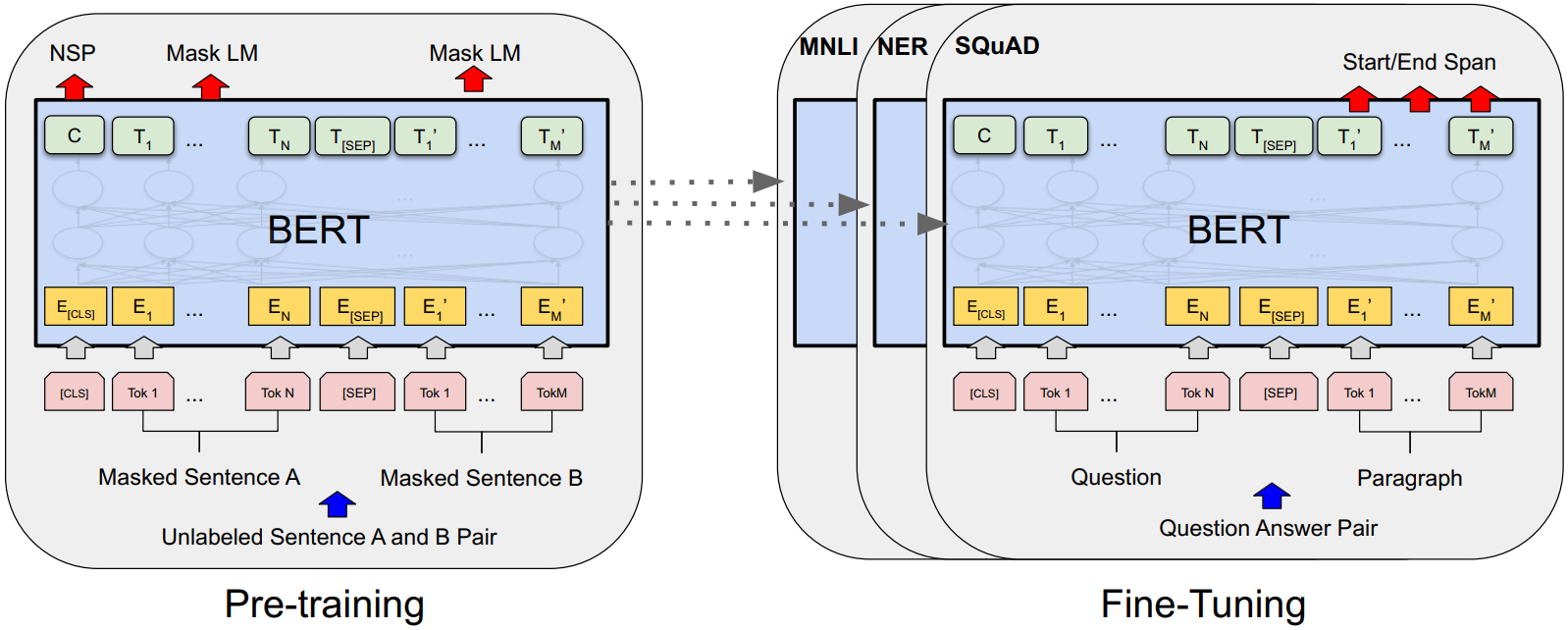
Figure 1: BERT pre-training 和 fine-tuning 过程。预训练模型和微调模型的输出层不一样，除此之外的架构是一样的。
左：用无标注的句子进行预训练，得到一个基础模型（预训练模型）。
右：用同一个基础模型作为起点，针对不同的下游任务进行微调，这会影响模型的所有参数。
[CLS] 是加到每个输入开头的一个特殊 token； [SEP] 是一个特殊的 separator token (e.g. separating questions/answers)

BERT 的一个独特之处是针对不同任务使用统一架构。预训练架构和最终下游架构之间的差异非常小。

3.0.1 BERT 模型架构和参数

我们的实现基于 Vaswani 等（2017）的原始实现和我们的库 tensor2tensor 。 Transformer 大家已经耳熟能详，并且我们的实现几乎与原版相同，因此这里不再对架构背景做详细描述，需要补课的请参考 Vaswani 等（2017）及网上一些优秀文章，例如 The Annotated Transformer。

本文符号表示，

L 层数（i.e., Transformer blocks）
H 隐藏层大小（embedding size）
A self-attention head 数量

In all cases we set the feed-forward/filter size to be 4H, i.e., 3072 for the H = 768 and 4096 for the H = 1024.

本文主要给出两种尺寸的模型：

BERT_BASE（L=12，H=768，A=12，总参数=110M），参数与 OpenAI GPT 相同，便于比较；
BERT_LARGE（L=24，H=1024，A=16，总参数=340M）

如果不理解这几个参数表示什么意思，可参考 Transformer 是如何工作的：600 行 Python 代码实现两个（文本分类+文本生成）Transformer（2019）。译注。

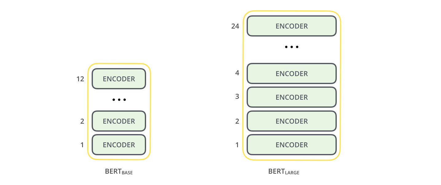
两个 size 的 BERT，图中的 encoder 就是 transformer。译注。Image Source

BERT Transformer 使用双向 self-attention，而 GPT Transformer 使用受限制的 self-attention，其中每个 token 只能关注其左侧的上下文。

We note that in the literature the bidirectional Transformer is often referred to as a “Transformer encoder” while the left-context-only version is referred to as a “Transformer decoder” since it can be used for text generation.

3.0.2 输入/输出表示

为了使 BERT 能够处理各种下游任务，在一个 token 序列中，我们的输入要能够明确地区分：

单个句子（a single sentence）
句子对（a pair of sentences）例如，问题/回答。

这里，

“句子”可以是任意一段连续的文本，而不是实际的语言句子。
“序列”是指输入给 BERT 的 token 序列，可以是单个句子或两个句子组合在一起。

我们使用 30,000 tokens vocabulary 的 WordPiece embeddings (Wu et al., 2016)。

这个 vocabulary 长什么样，可以可以看一下 bert-base-chinese（官方专门针对中文训练的基础模型）： bert-base-chinese/blob/main/vocab.txt。译注。

我们 input/output 设计如下：

每个序列的第一个 token 都是特殊的 classification token [CLS]；

在最终输出中（最上面一行），这个 token (hidden state) 主要用于分类任务，再接一个分类器就能得到一个分类结果（其他的 tokens 全丢弃），如下图所示，

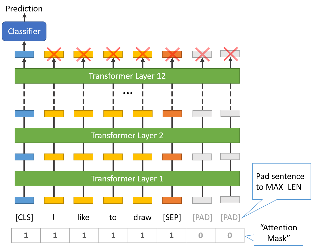
BERT 用于分类任务，classifier 执行 feed-forward + softmax 操作，译注。 Image Source
将 sentence-pair 合并成单个序列。通过两种方式区分，
1. 使用特殊 token [SEP] 来分隔句子；
2. 为每个 token 添加一个学习到的 embedding ，标识它属于句子 A 还是句子 B。

再回到图 1 所示，我们将

输入 embedding 表示为 $E$，

对于给定的 token ，它的输入表示是通过将相应的 token 、段落和位置 embedding 相加来构建的。图 2 可视化了这个构建过程，

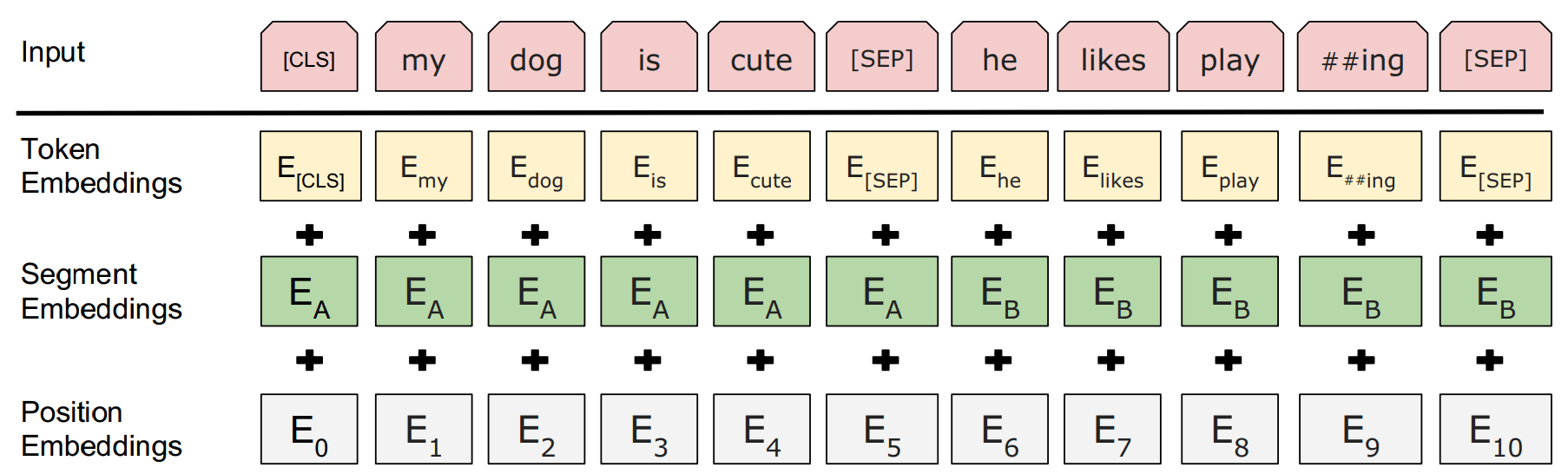
Figure 2: BERT input representation. input embeddings 是 token embeddings, segmentation embeddings 和 position embeddings 之和。
第 $i$ 个输入 token 的在最后一层的表示（最终隐藏向量）为 $T_i$，$T_i \in \mathbb{R}^H$。
[CLS] token 在最后一层的表示（最终隐藏向量）为 $C$, $C \in \mathbb{R}^{H}$ ，

3.1 预训练 BERT

图 1 的左侧部分。

Figure 1: BERT 的 pre-training 和 fine-tuning 过程。

与 Peters 等（2018a）和 Radford 等（2018）不同，我们不使用传统的从左到右或从右到左的模型来预训练 BERT，而是用下面两个无监督任务（unsupervised tasks）来预训练 BERT。

3.1.1 任务 `＃1`：掩码语言模型（Masked LM）

从直觉上讲，深度双向模型比下面两个模型都更强大：

从左到右的单向模型（LRM）；
简单拼接（shallow concatenation）了一个左到右模型（LRM）与右到左模型（RLM）的模型。

不幸的是，标准的条件语言模型（conditional language models）只能从左到右或从右到左进行训练，因为 bidirectional conditioning 会使每个单词间接地“看到自己”，模型就可以轻松地在 multi-layered context 中预测目标词。

为了训练一个深度双向表示，我们简单地随机屏蔽一定比例的输入 tokens，然后再预测这些被屏蔽的 tokens。我们将这个过程称为“掩码语言模型”（MLM） —— 这种任务通常也称为 Cloze（完形填空）（Taylor，1953）。

在所有实验中，我们随机屏蔽每个序列中 15% 的 token。与 denoising auto-encoders（Vincent 等，2008）不同，我们只预测被屏蔽的单词，而不是重建整个输入。

这种方式使我们获得了一个双向预训练模型，但造成了预训练和微调之间的不匹配，因为微调过程中不会出现 [MASK] token。为了减轻这个问题，我们并不总是用 [MASK] token 替换“掩码”单词：训练数据生成器（training data generator）随机选择 15%的 token positions 进行预测。如果选择了第 i 个 token ，我们将第 i 个 token 用以下方式替换：

80% 的概率用 [MASK] token 替换，
10% 的概率用 随机 token 替换，
10% 的概率 保持不变。

然后，使用 $Ti$ 来预测原始 token ，并计算交叉熵损失（cross entropy loss）。附录 C.2 中比较了这个过程的几个变种。

3.1.2 任务 `＃2`：下一句预测（Next Sentence Prediction, NSP）

许多重要的下游任务，如问答（Question Answering, QA）和自然语言推理（Natural Language Inference, NLI）都基于理解两个句子之间的关系，而语言建模（language modeling）并无法直接捕获这种关系。

为了训练一个能理解句子关系的模型，我们预先训练了一个二元的下一句预测任务（a binarized next sentence prediction task）：给定两个句子 A 和 B，判断 B 是不是 A 的下一句。

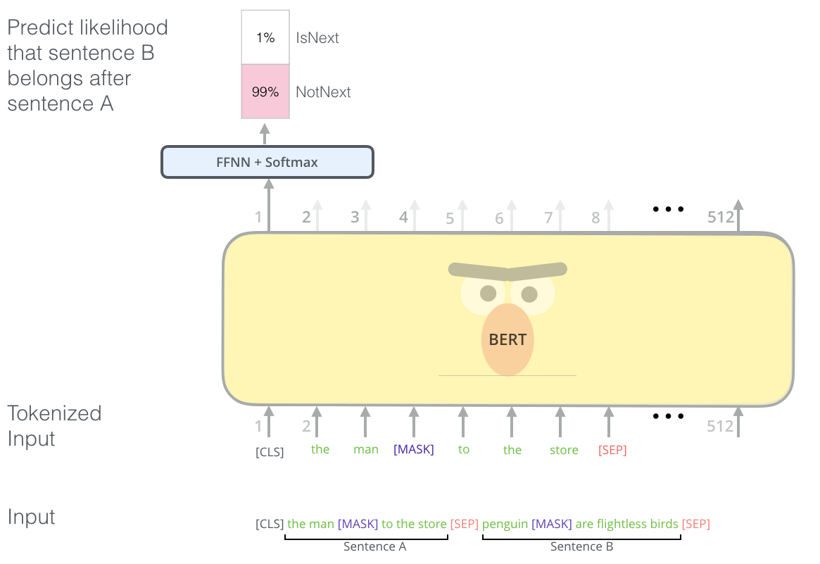
BERT 用于“下一句预测”（NSP）任务，译注。Image Source

这个任务可以用任何单语语料库（monolingual corpus），具体来说，在选择每个预训练示例的句子 A 和 B 时，

50％的概率 B 是 A 的下一个句子（labeled as IsNext），
50％的概率 B 是语料库中随机一个句子（labeled as NotNext）。

再次回到图 1，这个 yes/no 的判断还是通过 classifier token 的最终嵌入向量 $C$ 预测的，

最终我们的模型达到了 97~98% 的准确性。尽管它很简单，但我们在第 5.1 节中证明，针对这个任务的预训练对于 QA 和 NLI 都非常有益。

The vector C is not a meaningful sentence representation without fine-tuning, since it was trained with NSP。

NSP 任务与 Jernite 等（2017）和 Logeswaran 和 Lee（2018）使用的 representation learning 有紧密关系。但是他们的工作中只将句子 embedding 转移到了下游任务，而 BERT 是将所有参数都转移下游，初始化微调任务用的初始模型。

3.1.3 预训练数据集

预训练过程跟其他模型的预训练都差不多。对于预训练语料库，我们使用了

BooksCorpus (800M words) (Zhu et al., 2015)
English Wikipedia (2,500M words)。只提取文本段落，忽略列表、表格和标题。

使用文档语料库而不是像 Billion Word Benchmark（Chelba 等，2013）这样的 shuffled sentence-level 语料库非常重要，因为方便提取长连续序列。

3.2 微调 BERT

Transformer 中的 self-attention 机制允许 BERT 对任何下游任务建模 —— 无论是 single text 还是 text pairs —— 只需要适当替换输入和输出，因此对 BERT 进行微调是非常方便的。

对于 text-pair 类应用，一个常见的模式是在应用 bidirectional cross attention 之前，独立编码 text-pair ，例如 Parikh 等（2016）；Seo 等（2017）。

但 BERT 使用 self-attention 机制来统一预训练和微调这两个阶段，因为使用 self-attention 对 concatenated text-pair 进行编码，有效地包含了两个句子之间的 bidirectional cross attention。

对于每个任务，只需将任务特定的输入和输出插入到 BERT 中，并对所有参数进行端到端的微调。预训练阶段，input 句子 A 和 B 的关系可能是：

sentence pairs
hypothesis-premise pairs in entailment
question-passage pairs in question answering
文本分类或序列打标（sequence tagging）中的 degenerate text-? pair。

在输出端，

普通 token representations 送到 token-level 任务的输出层，例如 sequence tagging 或问答，
[CLS] token representation 用于分类，例如 entailment or sentiment analysis。

与预训练相比，微调的成本相对较低。从完全相同的预训练模型开始，本文中所有结果都可以在最多 1 小时内在单个 Cloud TPU 上复制，或者在 GPU 上几个小时内。第 4 节会介绍一些细节。更多细节见附录 A.5。

3.3 各种场景

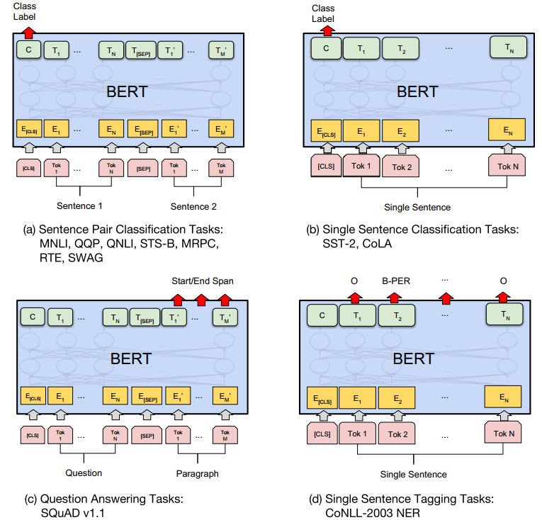
Fig 4. BERT 用于不同任务场景，来自 paper 附录。
(a) 句子对分类；(b) 单句分类；(c) 问答；(d) 单句打标。

In this section, we present BERT fine-tuning results on 11 NLP tasks.

4.1 GLUE (General Language Understanding Evaluation)

GLUE benchmark (Wang et al., 2018a) 是一个自然语言理解任务集，更多介绍见 Appendix B.1。

4.1.1 Fine-tune 工作

针对 GLUE 进行 fine-tune 所做的工作：

用第 3 节介绍的方式表示 input sequence (for single sentence or sentence pairs)
用 the final hidden vector C 判断类别；
fine-tuning 期间增加的唯一参数 是分类层的权重 $W \in \mathbb{R}^{K \times H}$，其中 $K$ 是 labels 数量。我们用 $C$ 和 $W$ 计算一个标准的 classification loss，例如 $\log({\rm softmax}(CW^T))$.

4.1.2 参数设置

batch size 32
3 epochs
learning rate: for each task, we selected the best fine-tuning learning rate (among 5e-5, 4e-5, 3e-5, and 2e-5) on the Dev set.

另外，我们发现 BERTLARGE 在小数据集上 finetuning 有时候不稳定，所以我们会随机重启几次，从得到的模型中选效果最好的。随机重启使用相同的 pre-trained checkpoint 但使用不同的数据重排和分类层初始化 （data shuffling and classifier layer initialization）。

4.1.3 结果

结果如 Table 1 所示，

System	MNLI-(m/mm)	QQP	QNLI	SST-2	CoLA	STS-B	MRPC	RTE	Average
	392k	363k	108k	67k	8.5k	5.7k	3.5k	2.5k	-
Pre-OpenAI SOTA	80.6/80.1	66.1	82.3	93.2	35.0	81.0	86.0	61.7	74.0
BiLSTM+ELMo+Attn	76.4/76.1	64.8	79.8	90.4	36.0	73.3	84.9	56.8	71.0
OpenAI GPT	82.1/81.4	70.3	87.4	91.3	45.4	80.0	82.3	56.0	75.1
BERTBASE	84.6/83.4	71.2	90.5	93.5	52.1	85.8	88.9	66.4	79.6
BERTLARGE	86.7/85.9	72.1	92.7	94.9	60.5	86.5	89.3	70.1	82.1

Table 1: GLUE Test results, scored by the evaluation server (https://gluebenchmark.com/leaderboard). The number below each task denotes the number of training examples. The “Average” column is slightly different than the official GLUE score, since we exclude the problematic WNLI set.8 BERT and OpenAI GPT are singlemodel, single task. F1 scores are reported for QQP and MRPC, Spearman correlations are reported for STS-B, and accuracy scores are reported for the other tasks. We exclude entries that use BERT as one of their components.

Both BERTBASE and BERTLARGE outperform all systems on all tasks by a substantial margin, obtaining 4.5% and 7.0% respective average accuracy improvement over the prior state of the art. Note that BERTBASE and OpenAI GPT are nearly identical in terms of model architecture apart from the attention masking. For the largest and most widely reported GLUE task, MNLI, BERT obtains a 4.6% absolute accuracy improvement. On the official GLUE leaderboard, BERTLARGE obtains a score of 80.5, compared to OpenAI GPT, which obtains 72.8 as of the date of writing.

We find that BERTLARGE significantly outperforms BERTBASE across all tasks, especially those with very little training data. The effect of model size is explored more thoroughly in Section 5.2.

4.2 SQuAD (Stanford Question Answering Dataset) v1.1

SQuAD v1.1 包含了 100k crowdsourced question/answer pairs (Rajpurkar et al., 2016). Given a question and a passage from Wikipedia containing the answer, the task is to predict the answer text span in the passage.

As shown in Figure 1, in the question answering task, we represent the input question and passage as a single packed sequence, with the question using the $A$ embedding and the passage using the $B$ embedding. We only introduce a start vector $S \in \mathbb{R}^H$ and an end vector $E \in \mathbb{R}^H$ during fine-tuning. The probability of word $i$ being the start of the answer span is computed as a dot product between $T_i$ and $S$ followed by a softmax over all of the words in the paragraph: $P_i = \frac{e^{S{\cdot}T_i}}{\sum_j e^{S{\cdot}T_j}}$. The analogous formula is used for the end of the answer span. The score of a candidate span from position $i$ to position $j$ is defined as $S{\cdot}T_i + E{\cdot}T_j$, and the maximum scoring span where $j \geq i$ is used as a prediction. The training objective is the sum of the log-likelihoods of the correct start and end positions. We fine-tune for 3 epochs with a learning rate of 5e-5 and a batch size of 32.

Table 2 shows top leaderboard entries as well as results from top published systems (Seo et al., 2017; Clark and Gardner, 2018; Peters et al., 2018a; Hu et al., 2018).

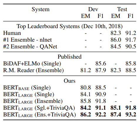
Table 2: SQuAD 1.1 results. The BERT ensemble is 7x systems which use different pre-training checkpoints and fine-tuning seeds.

The top results from the SQuAD leaderboard do not have up-to-date public system descriptions available,11 and are allowed to use any public data when training their systems. We therefore use modest data augmentation in our system by first fine-tuning on TriviaQA (Joshi et al., 2017) befor fine-tuning on SQuAD. Our best performing system outperforms the top leaderboard system by +1.5 F1 in ensembling and +1.3 F1 as a single system. In fact, our single BERT model outperforms the top ensemble system in terms of F1 score. Without TriviaQA fine- tuning data, we only lose 0.1-0.4 F1, still outperforming all existing systems by a wide margin.12

4.3 SQuAD v2.0

The SQuAD 2.0 task extends the SQuAD 1.1 problem definition by allowing for the possibility that no short answer exists in the provided paragraph, making the problem more realistic. We use a simple approach to extend the SQuAD v1.1 BERT model for this task. We treat questions that do not have an answer as having an answer span with start and end at the [CLS] token. The probability space for the start and end answer span positions is extended to include the position of the [CLS] token.

For prediction, we compare the score of the no-answer span: $s_{\tt null} = S{\cdot}C + E{\cdot}C$ to the score of the best non-null span $\hat{s_{i,j}}$ = ${\tt max}_{j \geq i} S{\cdot}T_i + E{\cdot}T_j$. We predict a non-null answer when $\hat{s_{i,j}} > s_{\tt null} + \tau$, where the threshold $\tau$ is selected on the dev set to maximize F1. We did not use TriviaQA data for this model. We fine-tuned for 2 epochs with a learning rate of 5e-5 and a batch size of 48.

The results compared to prior leaderboard entries and top published work (Sun et al., 2018; Wang et al., 2018b) are shown in Table 3, excluding systems that use BERT as one of their components. We observe a +5.1 F1 improvement over the previous best system.

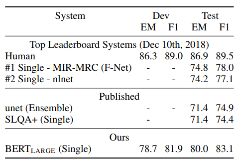
Table 3: SQuAD 2.0 results. We exclude entries that use BERT as one of their components.

4.4 SWAG (Situations With Adversarial Generations)

SWAG dataset contains 113k sentence-pair completion examples that evaluate grounded commonsense inference (Zellers et al., 2018).

Given a sentence, the task is to choose the most plausible continuation among four choices. When fine-tuning on the SWAG dataset, we construct four input sequences, each containing the concatenation of the given sentence (sentence A) and a possible continuation (sentence B). The only task-specific parameters introduced is a vector whose dot product with the [CLS] token representation C denotes a score for each choice which is normalized with a softmax layer.

We fine-tune the model for 3 epochs with a learning rate of 2e-5 and a batch size of 16. Results are presented in Table 4.

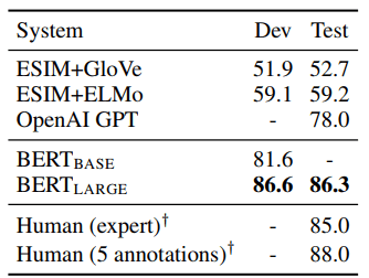
Table 4: SWAG Dev and Test accuracies. Human performance is measured with 100 samples, as reported in the SWAG paper.

BERTLARGE outperforms the authors’ baseline ESIM+ELMo system by +27.1% and OpenAI GPT by 8.3%.

本节研究去掉 BERT 的一些功能，看看在不同任务上性能损失多少，

sentence-level (e.g., SST-2)
sentence-pair-level (e.g., MultiNLI)
word-level (e.g., NER)
span-level (e.g., SQuAD)

以更好地理解它们的相对重要性。更多相关信息见附录 C。

5.1 预训练任务（MLM/NSP）的影响

5.1.1 训练组

通过以下几组来验证 BERT 深度双向性的重要性，它们使用与 BERTBASE 完全相同的预训练数据、微调方案和超参数：

NO NSP：即去掉“下一句预测”任务，这仍然是一个双向模型，使用“掩码语言模型”（MLM）进行训练，只是训练时不做 NSP 任务；
LTR & NO NSP：不仅去掉 NSP，还使用标准的从左到右（Left-to-Right, LTR）模型进行训练，而非使用双向模型。在微调中也遵从 left-only 约束，否则会导致预训练和微调不匹配，降低下游性能。此外，该模型没有用 NSP 任务进行预训练。这与 OpenAI GPT 直接可比，但我们使用了更大的训练数据集、我们自己的输入表示和我们的微调方案。
+ BiLSTM：在 fine-tuning 期间，在 LTR & NO NSP 基础上添加了一个随机初始化的 BiLSTM。

5.1.2 结果对比

结果如表 5，

Tasks	MNLI-m (Acc)	QNLI (Acc)	MRPC (Acc)	SST-2 (Acc)	SQuAD (F1)
BERTBASE	84.4	88.4	86.7	92.7	88.5
No NSP	83.9	84.9	86.5	92.6	87.9
LTR & No NSP	82.1	84.3	77.5	92.1	77.8
+ BiLSTM	82.1	84.1	75.7	91.6	84.9

Table 5: Ablation over the pre-training tasks using the BERTBASE architecture.

分析：

第二组 vs 第一组：去掉 NSP 任务带来的影响：在 QNLI、MNLI 和 SQuAD 1.1 上性能显著下降。
第三组 vs 第二组：去掉双向表示带来的影响：第二行实际上是 MLM & NO NSP，可以看出 LTR 模型在所有任务上的表现都比 MLM 模型差，尤其是 MRPC 和 SQuAD。
- 对于 SQuAD，可以清楚地看到 LTR 模型在 token 预测上表现不佳，因为 token 级别的隐藏状态没有右侧上下文。
- 为了尝试增强 LTR 系统，我们在其上方添加了一个随机初始化的双向 LSTM。这确实在 SQuAD 上改善了结果，但结果仍远远不及预训练的双向模型。另外，双向 LSTM 降低了在 GLUE 上的性能。

5.1.3 与 ELMo 的区别

ELMo 训练了单独的从左到右（LTR）和从右到左（RTL）模型，并将每个 token 表示为两个模型的串联。然而：

这比单个双向模型训练成本高一倍；
对于像 QA 这样的任务，这不直观，因为 RTL 模型将无法 condition the answer on the question；
这比深度双向模型弱，因为后者可以在每层使用左右上下文。

5.2 模型大小的影响

为探讨模型大小对微调任务准确性的影响，我们训练了多个 BERT 模型。表 6 给出了它们在 GLUE 任务上的结果。

L (层数)	H (hidden size)	A (attention head 数)	LM (ppl)	MNLI-m	MRPC	SST-2
3	768	12	5.84	77.9	79.8	88.4
6	768	3	5.24	80.6	82.2	90.7
6	768	12	4.68	81.9	84.8	91.3
12	768	12	3.99	84.4	86.7	92.9
12	1024	16	3.54	85.7	86.9	93.3
24	1024	16	3.23	86.6	87.8	93.7

Table 6: Ablation over BERT model size. “LM (ppl)” is the masked LM perplexity of held-out training data

In this table, we report the average Dev Set accuracy from 5 random restarts of fine-tuning.

可以看到，更大的模型在四个数据集上的准确性都更高 —— 即使对于只有 3,600 个训练示例的 MRPC，而且这个数据集与预训练任务差异还挺大的。也许令人惊讶的是，在模型已经相对较大的前提下，我们仍然能取得如此显著的改进。例如，

Vaswani 等（2017）尝试的最大 Transformer 是（L=6，H=1024，A=16），编码器参数为 100M，
我们在文献中找到的最大 Transformer 是（L=64，H=512，A=2），具有 235M 参数（Al-Rfou 等，2018）。
相比之下，BERTBASE 包含 110M 参数，BERTLARGE 包含 340M 参数。

业界早就知道，增加模型大小能持续改进机器翻译和语言建模等大规模任务上的性能，表 6 的 perplexity 列也再次证明了这个结果，然而，我们认为 BERT 是第一个证明如下结果的研究工作：只要模型得到了充分的预训练，那么将模型尺寸扩展到非常大时（scaling to extreme model sizes）， 对非常小规模的任务（very small scale tasks）也能带来很大的提升（large improvements）。

另外，

Peters 等（2018b）研究了将 pre-trained bi-LM size（预训练双向语言模型大小）从两层增加到四层，对下游任务产生的影响，
Melamud 等（2016）提到将隐藏维度从 200 增加到 600 有所帮助，但进一步增加到 1,000 并没有带来更多的改进。

这两项工作都使用了基于特征的方法，而我们则是直接在下游任务上进行微调，并仅使用非常少量的随机初始化附加参数，结果表明即使下游任务数据非常小，也能从更大、更 expressive 的预训练表示中受益。

5.3 BERT 基于特征的方式

到目前为止，本文展示的所有 BERT 结果都使用的微调方式：在预训练模型中加一个简单的分类层，针对特定的下游任务对所有参数进行联合微调。

5.3.1 基于特征的方式适用的场景

不过，基于特征的方法 —— 从预训练模型中提取固定特征（fixed features）—— 在某些场景下有一定的优势，

首先，不是所有任务都能方便地通过 Transformer encoder 架构表示，因此这些不适合的任务，都需要添加一个 task-specific model architecture。
其次，昂贵的训练数据表示（representation of the training data）只预训练一次，然后在此表示的基础上使用更轻量级的模型进行多次实验，可以极大节省计算资源。

5.3.2 实验

本节通过 BERT 用于 CoNLL-2003 Named Entity Recognition (NER) task (Tjong Kim Sang and De Meulder, 2003) 来比较这两种方式。

BERT 输入使用保留大小写的 WordPiece 模型，并包含数据提供的 maximal document context。
按照惯例，我们将其作为打标任务（tagging task），但在输出中不使用 CRF 层。
我们将第一个 sub-token 的 representation 作 token-level classifier 的输入，然后在 NER label set 上进行实验。

为了对比微调方法的效果，我们使用基于特征的方法，对 BERT 参数不做任何微调，而是从一个或多个层中提取激活（extracting the activations）。这些 contextual embeddings 作为输入，送给一个随机初始化的 two-layer 768-dimensional BiLSTM，最后再送到分类层。

5.3.3 结果

结果见表 7。BERTLARGE 与业界最高性能相当，

System	Dev F1	Test F1
ELMo (Peters et al., 2018a)	95.7	92.2
CVT (Clark et al., 2018)	-	92.6
CSE (Akbik et al., 2018)	-	93.1
`Fine-tuning approach`
BERTLARGE	96.6	92.8
BERTBASE	96.4	92.4
`Feature-based approach (BERTBASE)`
Embeddings	91.0	-
Second-to-Last Hidden	95.6	-
Last Hidden	94.9	-
Weighted Sum Last Four Hidden	95.9	-
Concat Last Four Hidden	96.1	-
Weighted Sum All 12 Layers	95.5	-

Table 7: CoNLL-2003 Named Entity Recognition results. Hyperparameters were selected using the Dev set. The reported Dev and Test scores are averaged over 5 random restarts using those hyperparameters

The best performing method concatenates the token representations from the top four hidden layers of the pre-trained Transformer, which is only 0.3 F1 behind fine-tuning the entire model.

这表明 微调和基于特征的方法在 BERT 上都是有效的。

Recent empirical improvements due to transfer learning with language models have demonstrated that rich, unsupervised pre-training is an integral part of many language understanding systems. In particular, these results enable even low-resource tasks to benefit from deep unidirectional architectures.

Our major contribution is further generalizing these findings to deep bidirectional architectures, allowing the same pre-trained model to successfully tackle a broad set of NLP tasks.

A. Additional Details for BERT

A.1 Illustration of the Pre-training Tasks

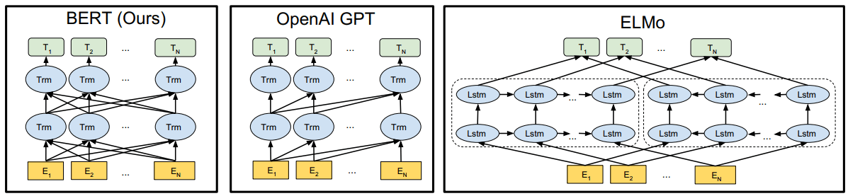
Figure 3: Differences in pre-training model architectures. BERT uses a bidirectional Transformer. OpenAI GPT uses a left-to-right Transformer. ELMo uses the concatenation of independently trained left-to-right and right-toleft LSTMs to generate features for downstream tasks. Among the three, only BERT representations are jointly conditioned on both left and right context in all layers. In addition to the architecture differences, BERT and OpenAI GPT are fine-tuning approaches, while ELMo is a feature-based approach.

A.2 Pre-training Procedure

A.3 Fine-tuning Procedure

For fine-tuning, most model hyperparameters are the same as in pre-training, with the exception of the batch size, learning rate, and number of training epochs. The dropout probability was always kept at 0.1. The optimal hyperparameter values are task-specific, but we found the following range of possible values to work well across all tasks:

Batch size: 16, 32
Learning rate (Adam): 5e-5, 3e-5, 2e-5
Number of epochs: 2, 3, 4

We also observed that large data sets (e.g., 100k+ labeled training examples) were far less sensitive to hyperparameter choice than small data sets. Fine-tuning is typically very fast, so it is reasonable to simply run an exhaustive search over the above parameters and choose the model that performs best on the development set.

A.4 Comparison of BERT, ELMo ,and OpenAI GPT

A.5 Illustrations of Fine-tuning on Different Tasks

B. Detailed Experimental Setup