Table of Links

Abstract and Intro

Related work

Approaches

Hyperparameter optimization

Estimating the number of novel classes

Full training procedure

Experiments

Conclusion

Declarations

References

Appendix A: Additional result metrics

Appendix B: Hyperparameters

Appendix C: Cluster Validity Indices numerical results

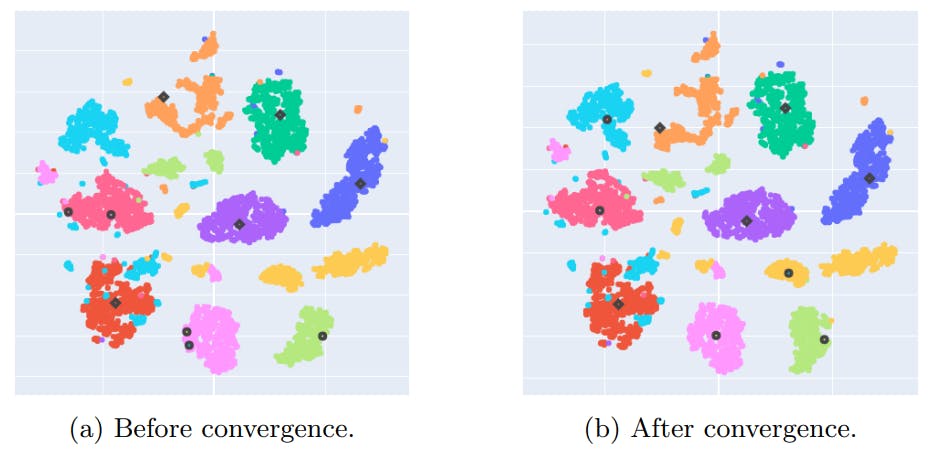
Appendix D: NCD k-means centroids convergence study

3 Approaches

In this section, after introducing the notations, we define two simple but potentially strong models derived from classical clustering algorithms (Sections 3.2 and 3.3). The idea is to use the labeled data to improve the unsupervised clustering process, and make the comparison to NCD methods more challenging. Then, we present a new method, PBN (for Projection-Based NCD, Section 3.4), characterized by its low number of hyperparameters needed to be tuned.

3.1 Problem setting

3.2 NCD k-means

This is a straightforward method that takes inspiration from k-means++ [24], which is an algorithm for choosing the initial positions of the centroids (or cluster centers). In k-means++, the first centroid is chosen at random from the data points. Then, each new centroid is chosen iteratively from one of the data points with a probability proportional to the squared distance from the point’s closest centroid. The resulting initial positions of the centroids are generally spread more evenly, which yields appreciable improvement in the final error of k-means and convergence time.

Similarly to k-means++, we repeat the initialization process a few times and keep the centroids that achieved the smallest inertia. Note that, to stay consistent with the

k-means algorithm, we use also the L2 norm (i.e. the Euclidean distance) for NCD k-means.

3.3 NCD Spectral Clustering

To incorporate the knowledge from the known classes in the Spectral Clustering process, our initial approach was to utilize NCD k-means within the spectral embedding. In short, we would initially compute the full spectral embedding for all the data and determine the mean points of the known classes with the help of the ground truth labels. These mean points would then serve as the initial centroids. However, the observed performance improvement over the fully unsupervised SC was quite marginal.

Instead, the idea that we will use throughout this article (and that we refer to as “NCD Spectral Clustering”) stems from the observation that SC can obtain very different results according to the parameters that are used. Among these parameters, the temperature parameter σ of the kernel holds particular importance, as it directly impacts the adjacency matrix’s accuracy in representing the neighborhood relationships of the data points. The rule of thumb of Equation 1 still requires to choose a value, but significantly reduces the space of possible values. Additionally, while the literature often sets the number of components u of the spectral embedding equal to the number of clusters, we have observed that optimizing it can also improve performance.

Therefore, rather than a specific method, we propose the parameter optimization scheme illustrated in Figure 2. For a given combination of parameters {smin, u}, the

corresponding spectral embedding of all the data is computed and then partitioned with k-means. The quality of the parameters is evaluated from the clustering performance on the known classes, as the ground-truth labels are only available for the known classes. Indeed an important hypothesis behind the NCD setup is that the known and novel classes are related and share similarities, so they should have similar feature scales and distributions. Consequently, if the Spectral Clustering performs well on the known classes, the parameters are likely suitable to represent the novel classes.

Discussion. This idea can be applied to optimize the parameters of any unsupervised clustering algorithm in the NCD context. For example, the Eps and M inP ts parameters of DBSCAN [29] can be selected in the same manner. It is also possible to use a different adjacency matrix in the SC algorithm. One option could be to substitute the Gaussian kernel with the k-nearest neighbor graph, and therefore optimise k instead of σ. However, for the sake of simplicity, we will only investigate SC using the Gaussian kernel.

3.4 Projection-Based NCD

The cross-entropy loss on the known classes is defined as:

The reconstruction loss of the instances from all classes is written as:

Projection-based NCD requires tuning of four hyperparameters. The trade-off parameter w is inherent to the method and the other three come from the choice of architecture: the learning rate, the dropout rate and the size of the latent space.

Note that this method doesn’t employ complex schemes to define pseudo-labels unlike many NCD works. They have been proven to be accurate with image data (notably thanks to data augmentation techniques) [4, 31], but we found in preliminary results not detailed here, that for tabular data, they introduce variability in the results and new hyperparameters that need to be tuned.

3.5 Summary of proposed approaches

In the next section, we present an approach to finding hyperparameters without using the labels of the novel classes, which are not available in realistic scenarios. Indeed in the experiments (see Section 7), it should become clear why the simplicity of the proposed approach is a desirable feature for hyperparameter optimization in the NCD context.