2021-10-16 02:29:24 Author: research.nccgroup.com(查看原文) 阅读量:21 收藏
Outline
- 1. Introduction
- 2. How does xorshift128 PRNG work?
- 3. Neural Networks and XOR gates
- 4. Using Neural Networks to model the xorshift128 PRNG
- 5. Creating a machine-learning-resistant version of xorshift128
- 6. Conclusion
1. Introduction
This blog post proposes an approach to crack Pseudo-Random Number Generators (PRNGs) using machine learning. By cracking here, we mean that we can predict the sequence of the random numbers using previously generated numbers without the knowledge of the seed. We started by breaking a simple PRNG, namely XORShift, following the lead of the post published in [1]. We simplified the structure of the neural network model from the one proposed in that post. Also, we have achieved a higher accuracy. This blog aims to show how to train a machine learning model that can reach 100% accuracy in generating random numbers without knowing the seed. And we also deep dive into the trained model to show how it worked and extract useful information from it.
In the mentioned blog post [1], the author replicated the xorshift128 PRNG sequence with high accuracy without having the PRNG seed using a deep learning model. After training, the model can use any consecutive four generated numbers to replicate the same sequence of the PRNG with bitwise accuracy greater than 95%. The details of this experiment’s implementation and the best-trained model can be found in [2].
At first glance, this seemed a bit counter-intuitive as the whole idea behind machine learning algorithms is to learn from the patterns in the data to perform a specific task, ranging from supervised, unsupervised to reinforcement learning. On the other hand, the pseudo-random number generators’ main idea is to generate random sequences and, hence, these sequences should not follow any pattern. So, it did not make any sense (at the beginning) to train an ML model, which learns from the data patterns, from PRNG that should not follow any pattern. Not only learn, but also get a 95% bitwise accuracy, which means that the model will generate the PRNG’s exact output and only gets, on average, two bits wrong. So, how is this possible? And why can machine learning crack the PRNG? Can we even get better than the 95% bitwise accuracy? That is what we are going to discuss in the rest of this article. Let’s start first by examining the xorshift128 algorithm.
** Editor’s Note: How does this relate to security? While this research looks at a non-cryptographic PRNG, we are interested, generically, in understanding how deep learning-based approaches to finding latent patterns within functions presumed to be generating random output could work, as a prerequisite to attempting to use deep learning to find previously-unknown patterns in cryptographic (P)RNGs, as this could potentially serve as an interesting supplementary method for cryptanalysis of these functions. Here, we show our work in beginning to explore this space. **
2. How does xorshift128 PRNG work?
To understand whether machine learning (ML) could crack the xorshift128 PRNG, we need to comprehend how it works and check whether it is following any patterns or not. Let’s start by digging into its implementation of the xorshift128 PRNG algorithm to learn how it works. The code implementation of this algorithm can be found on Wikipedia and shared in [2]. Here is the function that was used in the repo to generate the PRNG sequence (which is used to train the ML model):
def xorshift128():
    '''xorshift
    https://ja.wikipedia.org/wiki/Xorshift
    '''

    x = 123456789
    y = 362436069
    z = 521288629
    w = 88675123

    def _random():
        nonlocal x, y, z, w
        t = x ^ ((x << 11) & 0xFFFFFFFF)  # 32bit
        x, y, z = y, z, w
        w = (w ^ (w >> 19)) ^ (t ^ (t >> 8))
        return w

    return _random
As we can see from the code, the implementation is straightforward. It has four internal numbers, x, y, z, and w, representing the seed and the state of the PRNG simultaneously. Of course, we can update this generator implementation to provide the seed with a different function call instead of hardcoding it. Every time we call the generator, it will shift the internal variables as follows: y → x, z → y, and w → z. The new value of w is evaluated by applying some bit manipulations (shifts and XORs) to the old values of x and w. The new w is then returned as the new random number output of the random number generator. Let’s call the function output, o.
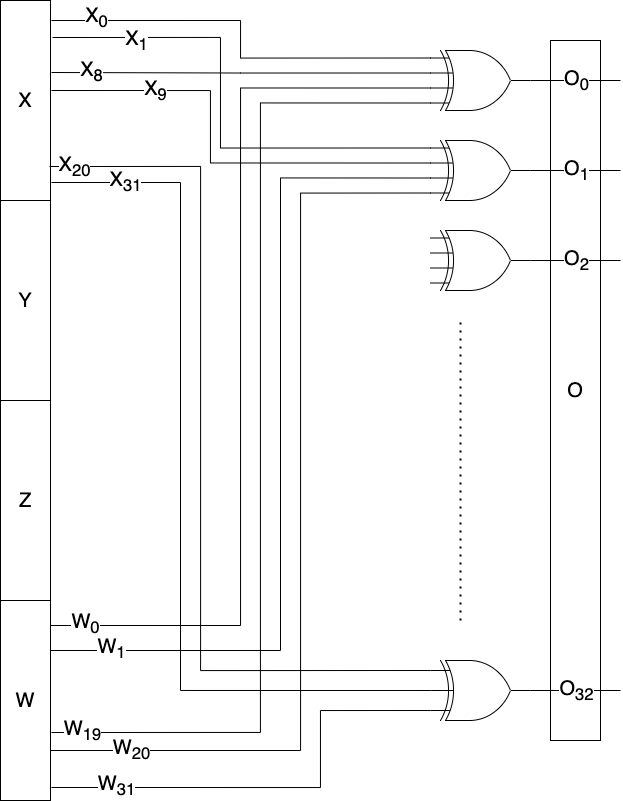
Using this code, we can derive the logical expression of each bit of the output, which leads us to the following output bits representations of the output, o:
O0 = W0 ^ W19 ^ X0 ^ X8
O1 = W1 ^ W20 ^ X1 ^ X9
.
.
O31 = W31 ^ X20 ^ X31
where Oi is the ith bit of the output, and the sign ^ is a bitwise XOR. The schematic diagram of this algorithm is shown below:

We can notice from this algorithm that we only need w and x to generate the next random number output. Of course, we need y and z to generate the random numbers afterward, but the value of o depends only on x and w.
So after understanding the algorithm, we can see the simple relation between the last four generated numbers and the next one. Hence, if we know the last four generated numbers from this PRNG, we can use the algorithm to generate the whole sequence; this could be the main reason why this algorithm is not cryptographically secure. Although the algorithm-generated numbers seem to be random with no clear relations between them, an attacker with the knowledge of the algorithm can predict the whole sequence of xorshift128 using any four consecutive generated numbers. As the purpose of this post is to show how an ML model can learn the hidden relations in a sample PRNG, we will assume that we only know that there is some relation between the newly generated number and its last four ones without knowing the implementation of the algorithm.
Returning to the main question slightly: Can machine learning algorithms learn to generate the xorshift128 PRNG sequence without knowing its implementation using only the last four inputs?
To answer this question, let’s first introduce the Artificial Neural Networks (ANN or NN for short) and how they may model the XOR gates.
3. Neural Networks and XOR gates
Neural Networks (NN), aka Multi-Layer Perceptron (MLP), is one of the most commonly used machine learning algorithms. It consists of small computing units, called neurons or perceptrons, organized into sets of unconnected neurons, called layers. The layers are interconnected to form paths from the inputs of the NN to its outputs. The following figure shows a simple example of 2 layers NN (the input layer is not counted). The details of the mathematical formulation of the NN are out of the scope of this article.

While the NN is being trained from the input data, the connections between the neurons, aka the weights, either get stronger (high positive or low negative values) to represent a high positively/negatively strong connection between two neurons or get weaker (close to 0) to represent that there is no connection at all. At the end of the training, these connections/weights encode the knowledge stored in the NN model.
One example used to describe how NNs handle nonlinear data is NN’s use to model a two-input XOR gate. The main reason for choosing the two-input XOR function is that although it is simple, its outputs are not linearly separable [3]. Hence, using an NN with two layers is the best way to represent the two input XOR gate. The following figure (from Abhranil blog [3]) shows how we can use a two-layer neural network to imitate a two-input XOR. The numbers on the lines are the weights, and the number inside the nodes are the thresholds (negative bias) and assuming using a step activation function.

In case we have more than two inputs for XOR, we will need to increase the number of the nodes in the hidden layer (the layer in the middle) to make it possible to represents the other components of the XOR.
4. Using Neural Networks to model the xorshift128 PRNG
Based on what we discussed in the previous section and our understanding of how the xorshift128 PRNG algorithm works, it makes sense now that ML can learn the patterns the xorshift128 PRNG algorithm follows. We can also now decide how to structure the neural network model to replicate the xorshift128 PRNG algorithm. More specifically, we will use a dense neural network with only one hidden layer as that is all we need to represent any set of XOR functions as implemented in the xorshift128 algorithm. Contrary to the model suggested in [1], we don’t see any reason to use a complex model like LSTM (“Long short-term memory,” a type of recurrent neural network), especially that all output bits are directly connected to sets of the input bits with XOR functions, as we have shown earlier, and there is no need for preserving internal states, as it is done in the LSTM.
4.1 Neural Network Model Design
Our proposed model would have 128 inputs in the input layer to represent the last four generated integer numbers, 32-bit each, and 32 outputs in the output layer to express the next 32-bit random generated number. The main hyperparameter that we need to decide is the number of neurons/nodes in the hidden layer. We don’t want a few nodes that can not represent all the XOR functions terms, and at the same time, we don’t want to use a vast number of nodes that would not be used and would complex the model and increase the training time. In this case, and based on the number of inputs, outputs, and the XOR functions complexity, we made an educated guess and used 1024 hidden nodes for the hidden layer. Hence, our neural network structure is as follows (the input layer is ignored):
_________________________________________________________________
Layer (type)                 Output Shape              Param #
=================================================================
dense (Dense)                (None, 1024)              132096
_________________________________________________________________
dense_1 (Dense)              (None, 32)                32800
=================================================================
Total params: 164,896
Trainable params: 164,896
Non-trainable params: 0
_________________________________________________________________
As we can see, the number of the parameters (weights and biases) of the hidden layer is 132,096 (128×1024 weights + 1024 biases), and the number of the parameters of the output layer is 32,800 (1024×32 weights + 32 biases), which gets to a total of 164,896 parameters to train. Comparing to the model used in [1]:
_________________________________________________________________
Layer (type)                 Output Shape              Param #
=================================================================
lstm (LSTM)                  (None, 1024)              4329472
_________________________________________________________________
dense (Dense)                (None, 512)               524800
_________________________________________________________________
dense_1 (Dense)              (None, 512)               262656
_________________________________________________________________
dense_2 (Dense)              (None, 512)               262656
_________________________________________________________________
dense_3 (Dense)              (None, 512)               262656
_________________________________________________________________
dense_4 (Dense)              (None, 512)               262656
_________________________________________________________________
dense_5 (Dense)              (None, 32)                16416
=================================================================
Total params: 5,921,312
Trainable params: 5,921,312
Non-trainable params: 0
_________________________________________________________________
This complex model has around 6 million parameters to train, which will make the model training harder and take a much longer time to get good results. It could also easily be stuck in one of the local minima in that huge 6 million dimension space. Additionally, storing this model and serving it later will use 36 times the space needed to store/serve our model. Furthermore, the number of the model parameters affects the amount of required data to train the model; the more parameters, the more input data is needed to train it.
Another issue with that model is the loss function used. Our target is to get as many correct bits as possible; hence, the most suitable loss function to be used in this case is “binary_crossentropy,” not “mse.” Without getting into the math of both of these loss functions, it is sufficient to say that we don’t care if the output is 0.8, 0.9, or even 100. All we care about is that the value crosses some threshold to be considered one or not to be considered zero. Another non-optimal choice of the parameter in that model is the activation function of the output layer. As the output layer comprises 32 neurons, each representing a bit whose value should always be 0 or 1, the most appropriate activation function for these types of nodes is usually a sigmoid function. On the contrary, that model uses a linear activation function to output any value from -inf to inf. Of course, we can threshold those values to convert them to zeros and ones, but the training of that model will be more challenging and take more time.
For the rest of the hyperparameters, we have used the same as in the model in [1]. Also, we used the same input sample as the other model, which consists of around 2 million random numbers sampled from the above PRNG function for training, and 10,000 random numbers for testing. Training and testing random number samples are formed into a quadrable of consequent random numbers to be used as inputs to the model, and the next random number is used as an output to the model. It is worth mentioning that we don’t think we need that amount of data to reach the performance we reached; we just tried to be consistent with the referenced article. Later, we can experiment to determine the minimum data size sufficient to produce a well-trained model. The following table summarises the model parameters/ hyperparameters for our model in comparison with the model proposed in [1]:
| NN Model in [1] | Our Model | |
|---|---|---|
| Model Type | LSTM and Dense Network | Dense Network |
| #Layers | 7 | 2 |
| #Neurons | 1024 LSTM 2592 Dense | 1056 Dense |
| #Trainable Parameters | 5,921,312 (4,329,472 only from the LSTM layer) | 164,896 |
| Activation Functions | Hidden Layers: relu Output Layer: linear | Hidden Layer: relu Output Layer: sigmoid |
| Loss Function | mse | binary_crossentropy |
4.2 Model Results
After a few hours of model training and optimizing the hyperparameters, the NN model has achieved 100% bitwise training accuracy! Of course, we ran the test set through the model, and we got the same result with 100% bitwise accuracy. To be more confident about what we have achieved, we have generated a new sample of 100,000 random numbers with a different seed than those used to generate the previous data, and we got the same result of 100% bitwise accuracy. It is worth mentioning that although the referenced article achieved 95%+ bitwise accuracy, which looks like a promising result. However, when we evaluated the model accuracy (versus bitwise accuracy), which is its ability to generate the exact next random numbers without any bits flipped, we found that the model’s accuracy dropped to around 26%. Compared to our model, we have 100% accuracy. The 95%+ bitwise is not failing only on 2 bits as it may appear (95% of 32 bit is less than 2), but rather these 5% errors are scattered throughout 14 bits. In other words, although the referenced model has bitwise accuracy of 95%+, 18 bits only would be 100% correct, and on average, 2 bits out of the rest of the 14 bits would be altered by the model.
The following table summarizes the two model comparisons:
| NN Model in [1] | Our Model | |
|---|---|---|
| Bitwise Accuracy | 95% + | 100% |
| Accuracy | 26% | 100% |
| Bits could be Flipped (out of 32) | 14 | 0 |
In machine learning, getting 100% accuracy is usually not good news. It normally means either we don’t have a good representation of the whole dataset, we are overfitting the model for the sample data, or the problem is deterministic that it does not need machine learning. In our case, it is close to the third choice. The xorshift128 PRNG algorithm is deterministic; we need to know which input bits are used to generate output bits, but the function to connect them, XOR, is already known. So, in a way, this algorithm is easy for machine learning to crack. So, for this problem, getting a 100% accurate model means that the ML model has learned the bits connection mappings between the input and output bits. So, if we get any consequent four random numbers generated from this algorithm, the model will generate the random numbers’ exact sequence as the algorithm does, without knowing the seed.
4.3 Model Deep Dive
This section will deep dive into the model to understand more what it has learned from the PRNG data and if it matches our expectations.
4.3.1 Model First Layer Connections
As discussed in section 2, the xorshift128 PRNG uses the last four generated numbers to generate the new random number. More specifically, the implementation of xorshift128 PRNG only uses the first and last numbers of the four, called w and x, to generate the new random number, o. So, we want to check the weights that connect the 128 inputs, the last four generated numbers merged, from the input layer to the hidden layer, the 1024 hidden nodes, of our trained model to see how strong they are connected and hence we can verify which bits are used to generate the outputs. The following figure shows the value of weights on the y-axes connecting each input, in x-axes, to the 1024 hidden nodes in the hidden layer. In other words, each dot on the graph represents the weight from any of the hidden nodes to the input in the x-axes:

As we can see, very few of the hidden nodes are connected to one of the inputs, where the weight is greater than ~2.5 or less than ~-2.5. The rest of the nodes with low weights between -2 and 2 can be considered not connected. We can also notice that inputs between bit 32 and 95 are not connected to any hidden layers. This is because what we stated earlier that the implementation of xorshift128 PRNG uses only x, bits from 0 to 31, and w, bits from 96 to 127, from the inputs, and the other two inputs, y, and z representing bits from 32 to 95, are not utilized to generate the output, and that is exactly what the model has learned. This implies that the model has learned that pattern accurately from the data given in the training phase.
4.3.2 Model Output Parsing
Similar to what we did in the previous section, the following figure shows the weights connecting each output, in x-axes, to the 1024 hidden nodes in the hidden layer:

Like our previous observation, each output bit is connected only to a very few nodes from the hidden layer, maybe except bit 11, which is less decisive and may need more training to be less error-prone. What we want to examine now is how these output bits are connected to the input bits. We will explore only the first bit here, but we can do the rest the same way. If we focus only on bit 0 on the figure, we can see that it is connected only to five nodes from the hidden layers, two with positive weights and three with negative weights, as shown below:

Those connected hidden nodes are 120, 344, 395, 553, and 788. Although these nodes look random, if we plot their connection to the inputs, we get the following figure:

As we can see, very few bits affect those hidden nodes, which we circled in the figure. They are bits 0, 8, 96, and 115, which if we modulo them by 32, we get bits 0 and 8 from the first number, x, and 0 and 19 from the fourth number, w. This matches the xorshift128 PRNG function we derived in section 2, the first bit of the output is the XOR of these bits, O0 = W0 ^ W19 ^ X0 ^ X8. We expect the five hidden nodes with the one output node to resemble the functionality of an XOR of these four input bits. Hence, the ML model can learn the XOR function of any set of arbitrary input bits if given enough training data.
5. Creating a machine-learning-resistant version of xorshift128
After analyzing how the xorshift128 PRNG works and how NN can easily crack it, we can suggest a simple update to the algorithm, making it much harder to break using ML. The idea is to introduce another variable in the seed that will decide:
- Which variables to use out of x, y, z, and w to generate o.
- How many bits to shift each of these variables.
- Which direction to shift these variables, either left or right.
This can be binary encoded in less than 32 bits. For example, only w and x variables generate the output in the sample code shown earlier, which can be binary encoded as 1001. The variable w is shifted 11 bits to the right, which can be binary encoded as 010110, where the least significant bit, 0, represents the right direction. The variable x is shifted 19 bits to the right, which can be binary encoded as 100111, where the least significant bit, 1, represents the left direction. This representation will take 4 bits + 4×6 bits = 28 bits. For sure, we need to make sure that the 4 bits that select the variables do not have these values: 0000, 0001, 0010, 0100, and 1000, as they would select one or no variable to XOR.
Using this simple update will add small complexity to PRNG algorithm implementation. It will still make the ML model learn only one possible sequence of about 16M different sequences generated with the same algorithm with different seeds. As if the ML would have only learned the seed of the algorithm, not the algorithm itself. Please note that the purpose of this update is to make the algorithm more resilient to ML attacks, but the other properties of the outcome PRNG, such as periodicity, are yet to be studied.
6. Conclusion
This post discussed how the xorshift128 PRNG works and how to build a machine learning model that can learn from the PRNG’s “randomly” generated numbers to predict them with 100% accuracy. This means that if the ML model gets access to any four consequent numbers generated from this PRNG, it can generate the exact sequence without getting access to the seed. We also studied how we can design an NN model that would represent this PRNG the best. Here are some of the lessons learned from this article:
- Although xorshift128 PRNG may to humans appear to not follow any pattern, machine learning can be used to predict the algorithm’s outputs, as the PRNG still follows a hidden pattern.
- Applying deep learning to predict PRNG output requires understanding of the specific underlying algorithm’s design.
- It is not necessarily the case that large and complicated machine learning models would attain higher accuracy that simple ones.
- Simple neural network (NN) models can easily learn the XOR function.
The python code for training and testing the model outlined in this post is shared in this repo in a form of a Jupyter notebook. Please note that this code is based on top of an old version of the code shared in the post in [1] with the changes explained in this post. This was intentionally done to keep the same data and other parameters unchanged for a fair comparison.
Acknowledgment
I would like to thank my colleagues in NCC Group for their help and support and for giving valuable feedback the especially in the crypto/cybersecurity parts. Here are a few names that I would like to thank explicitly: Ollie Whitehouse, Jennifer Fernick, Chris Anley, Thomas Pornin, Eric Schorn, and Marie-Sarah Lacharite.
References
[1] Everyone Talks About Insecure Randomness, But Nobody Does Anything About It
[2] The repo for code implementation for [1]
[3] https://blog.abhranil.net/2015/03/03/training-neural-networks-with-genetic-algorithms/
如有侵权请联系:admin#unsafe.sh